Implementation of Global Ensemble Forecast System (GEFS) at 12km Resolution

ISSN 0252-1075
 Contribution from IITM
 Technical Report No.TR-06
 ESSO/IITM/MM/TR/02(2020)/200

 Implementation of Global Ensemble Forecast
 System (GEFS) at 12km Resolution

Medha Deshpande, C.J. Johny, Radhika Kanase, Snehlata Tirkey, Sahadat Sarkar,
Tanmoy Goswami, Kumar Roy, Malay Ganai, R. Phani Murali Krishna, V.S. Prasad,
 P. Mukhopadhyay , V.R. Durai, Ravi S. Nanjundiah and M. Rajeevan

 Indian Institute of Tropical Meteorology (IITM)
 Ministry of Earth Sciences (MoES)
 PUNE, INDIA
 http://www.tropmet.res.in/

ISSN 0252-1075
 Contribution from IITM
 Technical Report No.TR-06
 ESSO/IITM/MM/TR/02(2020)/200

 Implementation of Global Ensemble Forecast
 System (GEFS) at 12km Resolution

 Medha Deshpande1, C.J. Johny2, RadhikaKanase1, Snehlata Tirkey1, Sahadat Sarkar1,
 Tanmoy Goswami1, Kumar Roy1, Malay Ganai1, R.Phani Murali Krishna1, V.S. Prasad2,
 P. Mukhopadhyay1 , V.R. Durai3, Ravi S. Nanjundiah1, 4and M. Rajeevan5

1
 Indian Institute of Tropical Meteorology, Ministry of Earth Sciences, Dr.Homi Bhabha Road, Pashan, Pune-
 411008
2
 National Centre for Medium Range Weather Forecasting, Ministry of Earth Sciences, A-50, Sector-62,
 NOIDA, UP
3
 India Meteorological Department, Ministry of Earth Sciences,MausamBhavan, Lodi Road, New Delhi
4
 Center for Atmospheric and Oceanic Sciences, Indian Institute of Science, Bengaluru - 560012
5
 Ministry of Earth Science, Government of India, PrithviBhavan, New Delhi

*Corresponding Author:
 Dr. P. Mukhopadhyay
 Indian Institute of Tropical Meteorology,
 Dr.Homi Bhabha Road, Pashan,
 Pune-411008, India.
 E-mail: mpartha@tropmet.res.in, parthasarathi64@gmail.com
 Phone: +91-(0)20-25904221

 Indian Institute of Tropical Meteorology (IITM)
 Ministry of Earth Sciences (MoES)
 PUNE, INDIA
 http://www.tropmet.res.in/

DOCUMENT CONTROL SHEET
----------------------------------------------------------------------------------------------------------------------------------
 Ministry of Earth Sciences (MoES)
 Indian Institute of Tropical Meteorology (IITM)

ESSO Document Number
ESSO/IITM/MM/TR/02(2020)/200

Title of the Report
Implementation of Global Ensemble Forecast System (GEFS) at 12km Resolution

Authors
Medha Deshpande1,C.J. Johny2, Radhika Kanase1, Snehlata Tirkey1, Sahadat Sarkar1, Tanmoy
Goswami1, Kumar Roy1, Malay Ganai1, R. Phani Murali Krishna1, V.S. Prasad2, P. Mukhopadhyay1 ,
V.R. Durai3, Ravi S. Nanjundiah1, 4and M. Rajeevan5

Type of Document
Technical Report

Number of pages and figures
26, 11

Number of references
15

Keywords
GEFS, Ensemble, EnKF, GFS, 12 Km, high-resolution

Security classification
Open

Distribution
Unrestricted

Date of Publication
August 2020

Abstract
To improve the weather forecasts and services across India, Global Ensemble Forecast System
(GEFS) model has been implemented on MoES HPCS system. The model has been ported on two
HPCS systems which has 21 ensembles (21) and runs at 12 Km resolution with 64 vertical levels.
The model runs twice a day on Operational mode. Various products are generated from this model
for the Indian region. This document gives a glimpse on the implementation of the GEFS model.

Summary

Many efforts are being done to increase the prediction skill of the high-impact weather systems
using the state-of-art models. With an intuition to improve the weather forecasts and services, we
have implemented Global Ensemble Forecast System (GEFS) model on the MoES HPCS system. The
high-resolution (~12Km) and the number of ensembles (21) make this GEFS system unique in the
world. This system is based on the deterministic GFS system of NCEP operationalized in 2018. The
initial conditions are generated from the Ensemble Kalman Filter (EnKF) method. The Ensemble
Transform methods are used to combine the perturbed ensembles and the ICs from the GDAS
assimilation system. Near Real-time SST (NSST) is also perturbed along with the other fields. 12Km
GEFS model suggests that the RMSE doesn’t change with the lead time. The model is able to
predict heavy precipitation events and the cyclonic storms more realistically. The EPSgram, Skew-T
plot and the QPF are very useful for the forecasters.

Contents

1. Introduction 1

2. Methodology 2

 2.1. Description of the model 2

 2.2. Computational details of the model 3

 2.3. Ensemble Kalman Filter (Data Assimilation) 4

3. Results and Discussion 5

 3.1. Verification of GEFS model with Probabilistic skill scores 5

 3.2. Ensemble mean features of GEFS model 6

 3.3. Tropical Cyclone Prediction 7

 3.4. Rainfall probability Forecasts at Block Level 7

 3.5. EPSgram 8

 3.6. Skew-T Plots 8

 3.7. QPF 9

4. Conclusions and Future works 9

5. Acknowledgements 10

6. References 10

7. Figures 11

1. Introduction

The scientific insights gained from the research work based on numerical experiments by

Smagorinsky, 1963; Leith, 1965; Mintz, 1965 and others in 1960s and further the epochal work of

Lorenz (1963) on limited predictability of deterministic forecast due to inherent chaotic nature of

the environment, have set the basis for ensemble prediction system (EPS). As a consequence to

these path breaking concepts, the EPS system for medium range forecast was established in

European Center for Medium Range Weather Forecast (ECMWF), UK (Buizza et al., 1993; Buizza

andPalmer, 1995) since 1992 (Palmer et al., 1992; Molteni et al., 1996). Contrary to the singular

vector approach of ECMWF, around same time NMC/NCEP, USA introduced the medium range

ensemble prediction system based on breeding vector approach (TothandKalnay, 1993; 1997). In

India, the ensemble prediction system for medium range weather was started at National Center for

Medium Range Weather Forecast (NCMRWF) at a moderate resolution of T190 in the year 2012

(Ashrit et al., 2012). However, with the pressing demand of stake holders and for different societal

needfor a forecast at higher resolution, Indian Institute of Tropical Meteorology implemented a

global high resolution (T1534~12.5km) ensemble prediction system with 21 ensemble members for

a ten day forecasts. This was done under the “Monsoon Mission” programme of Ministry of Earth

Sciences, Government of India in collaboration with NCMRWF for the perturbed initial conditions

and NCEP, USA for the model. The details of the model, porting and the perturbation techniques

are discussed in subsequent sections. The IITM GEFS system is operationalized by IMD on 1 June

2018. The current GEFS system is supposed to be the highest resolution global EPS system in the

world at present that is being used for 10 days forecast.

 1

2. Methodology

2.1 Description of GEFS model

Global Ensemble Forecast System (GEFS) was upgraded from ~27 km (T574 with GEFS v11.3) to
~12 km (T1534) resolution in year 2018. It is based on Global Forecast System (GFS v14.1) which
is a part of the „Operational Model‟ developed at NCEP, USA in 2018. Table 1.0 gives the
difference in the versions of the model which was newly implemented. The dynamics, horizontal
resolution, representation of physics processes and the Near surface SST (NSST) are among the few
to be mentioned which has significant changes in the new version. Apart from the more number of
observations, surface perturbations (NSST) are also included in the Initial Conditions (ICs). The
total number of 21 Ensembles (20 perturbed forecasts + 1 control forecast) constitutes the ensemble
system. These 20 ensembles analysis are generated by Ensemble Kalman Filter (EnKF) method
from the forecast perturbation of the previous cycles four times a day (00, 06, 12 and 18 UTC) at all
64 model vertical levels. These analysis perturbations are added to the reconfigured analysis
obtained from the hybrid four-dimensional Ensemble variational data assimilation system (GDAS-
Hybrid4DEnsVar) as part of the suite. The 243 hour forecast of GEFS is routinely generated based
on 00UTC and 12UTC initial conditions which include a control forecast starting from GDAS
assimilation and 20 (20 perturbations) ensemble members with each perturbed initial conditions.
Figure 1 gives the details of the 12Km GEFS model flow chart.

 Model Version V14.1.1.3 V11.1 (Older version)

 No. of ensembles members 20 + 1 20 +1

 No. of Levels (Sigma) 64 64
 a) Spectral model, with Semi- a) Spectral model with semi
 Lagrangian dynamics and Lagrangian dynamics
 Description about the Model
 Semi-implicit time scheme
 b) With Near surface SST
 Grid description Reduced Gaussian Linear Grid Reduced Gaussian Linear Grid

 Resolution T1534 (3072 x 1536) ~ 12.5KM T 574 (1152 x 576)
 Dynamics : 900 sec(450) Dynamics : 450 sec
 Model time-steps
 Physics : 450 sec(225) Physics : 225 sec
 Radiation time-steps 1 Hour for both LW and SW 1 Hour for both LW and SW
 Deep Convective Scale- and Aerosol-aware deep New- Simplified Arakawa
 Parameterization convection (SAS) Scheme
 Shallow Convective Scale- and Aerosol-aware shallow Mass-flux based Shallow
 parameterization scheme based on mass-flux convection
 Radiation RRTMG RRTM

 2

PBL EDMF EDMF

 Microphysics Zhao – Carr Microphysics Zhao – Carr Microphysics

 Surface Model NOAH Land Surface Model NOAH Land Surface Model
 243 Hours with 3 hourly interval 240 Hours with 6 hourly interval
 Forecast Length
 (cycles: 00UTC and 12 UTC) (only 00 UTC cycle)
 Initial Condition Perturbations Ensemble Kalman Filter (ENKF) Ensemble Kalman Filter (EnKF)
 Model I/O format Nemsio Sigma spectral
 Space requirement for 243 hrs
 21 TB / cycle 4 TB / cycle
 forecasts (21 ens)
 Post-Processing Grib2 Grib1

Table 1: GEFS T1534 model description and the older version of the model

2.2 Computational details of the Model

The GEFS model was made operational first at Pratyush HPCS of IITM and, later at Mihir HPCS of
NCMRWF. Pratyush and Mihir HPCS are Cray-XC40 Liquid Cooled System with 3315 nodes and
2320 nodes running with a peak performance of 4.006 PFand 2.8 +PF with a total system memory
of 414TB and 290 TB respectively. The deterministic model (GFS v14) takes around 90 minutes on
Cray XC-40 with 23 nodes. Out of the 23 nodes, 4nodes are used as I/O. Similarly, separate nodes
are allocated for writing the I/O as each ensemble writes nearly 10GB at each model output
frequency. The 21 member ensemble forecast takes nearly 90 minutes on 483 nodes of the same
system. Table 2 gives the specification of the complete details of the timing used for the GEFS
model.

 Wall Clock Number Details of
 Configuration Start Time
 Time (Minutes) of Nodes the run
 Global Ensemble Initialization (10) 0900, 2100 2 84 enkf.track
 Vortex Separation (12) After 10 2 84 init.seperate
 Ensemble Transform with Rescaling (13) After 12 10 84 init.et
 Ensemble Vortex Combine (14) After 13 20 84 init.combine
 Forecast (100) After 14 90 483 Fcst
 Post-Processing (102 – 182) After 100 20 540 ncep.post
 After Post
 Ensemble Average/Spread (194) 10 84 Ensstat
 processing
 After Ensemble
 Ensemble Tracker (396 – 397) 10 21 Gettrk
 average

Table 2: Timings/Nodes usage of the GEFS T1534 model. The number in the bracket indicates the
configuration number and the starting time depends on the completion of this number

 3

2.3 Ensemble Kalman Filter (Data assimilation)

 NCMRWF GFS data assimilation system employs hybrid Ensemble Variational (EnsVar)
technique with 80 member EnKF ensembles. The hybrid assimilation system is based on grid point
statistical interpolation (GSI), with background error covariance modified by inclusion of flow
dependent background error information from ensembles. In the background error, 87.5 %
contribution is provided by flow dependent error covariance and 12.5 % by static error covariance.
Here EnKF formulation uses ensemble square root filter (EnSRF) for generating ensembles as a part
of the hybrid GSI analysis system (Liu et al, 2015). EnKF uses observation operator in GSI to
compute observation innovations with respect to each ensemble. So all the observations used in the
GSI are available for assimilation in EnKF and observation selection and other quality control
procedures are done with in GSI operator. The assimilation system uses conventional and satellite
observations including many Indian observations. Table 3 gives details of observations used in
NCMRWF GSI assimilation system. In EnSRF formulations model analysis state is updated by
representing analysis variables as two terms, the ensemble mean and as a deviation from mean (Liu
et al, 2015). Ensemble analyses are re-centered around deterministic analysis from GSI using
recentering procedures and short forecasts are generated. The process is repeated 4 times a day
corresponding to 00, 06, 12 and 18 UTC. Twenty members of these EnKF ensembles are utilized in
GEFS forecasts utilizing different members in each cycle. At present GEFS is run at 00 UTC and 12
UTC using member 1-20 and 41-60 respectively.

Conventional observations Non Conventional observations
Tropical cyclone bogus MHS MLS ozone
Rawinsonde HIRS-4 OMPS (NP & TC8) ozone
PIBAL AIRS AHI
Dropsonde IASI GPSRO
AIREP SSM/IS UPP radiances AMV
 Scatterometer
AMDAR GOES sounder radiances
 (ASCAT/SCATSTAT)
U.S./Mexican/ADS-C
 SEVIRI/CSR GMI
MDCRS
Canadian AMDAR ATMS
S. American AMDAR CrIS
GPS-IPW (ground based) SAPHIR radiances
NPN wind profiler GOES imgr cloud products
VAD winds GOES sndr cloud products
JMA wind profile SBUV ozone
SYNOP METAR GOME ozone
Ship buoy platforms OMI ozone

 4

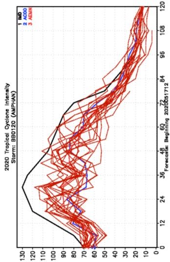
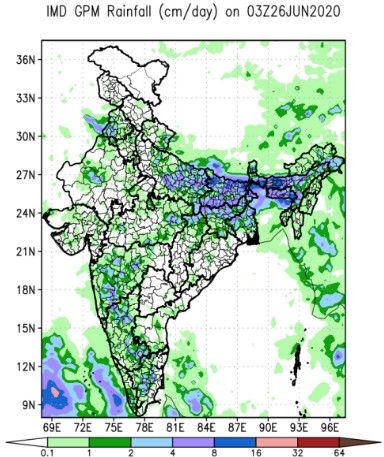
Table 3: Details of observations assimilated in GSI

3. Results and Discussion

 The new GEFS model at 12Km is operationalized on 01 June 2018. Many products are
generated from this model and are made available operationally at
https://srf.tropmet.res.in/srf/hires_gefs/index.php. Some of them and their skill scores are being
mentioned below.

3.1 Verification of GEFS with Probabilistic Skill scores

 To evaluate the statistical reliability of the ensemble forecast we have plotted the Root Mean

Square Error (RMSE) and spread of precipitation for June-September of 2018 and 2019 in Figure2.

RMSE of the ensemble mean measures the distance between forecast and IMD GPM Gridded

rainfall data. The spread measures the deviation of ensemble members from the ensemble mean. In

a perfect ensemble forecast system, where all of the uncertainties associated with initial errors and

model errors are represented, the verifying analysis is statistically indistinguishable from the

ensemble members and the spread would be equal to RMSE uncertainty (Zhu 2005, Buizza et al.

2005). The discrepancy between the RMSE of ensemble mean and ensemble spread is a measure of

the statistical reliability of an ensemble forecast system (Buizza et al. 2005). For a reliable ensemble

forecast system, this discrepancy should be low. The large difference between the two indicates

statistical inconsistency. For the Indian Landmass (Figure2)the spread is less than RMSE which

indicates precipitation forecast is under-dispersed. Also the growth in the RMSE is less than growth

in the spread with forecast lead time.

Brier Score (BS) is used for the verification of probabilistic forecasts (Brier 1950). It measures the
mean-square error between the probabilistic forecasts and the subsequent categorical observation. It
is given by,
 
 1
 = ( − )2
 
 =1

 5

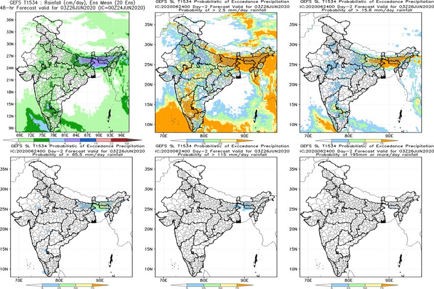
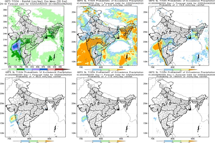
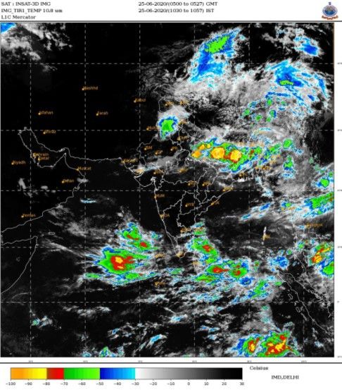
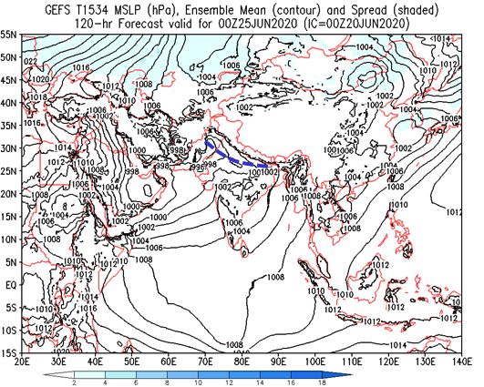
Where the difference is between the forecast probabilities and binary observations (ok=1, event
occurs and ok=0, event does not occur). The score ranges from 0 to 1 with 0 showing perfect
forecasts.
BS can be decomposed into reliability (REL), resolution (RES) and uncertainty (UNC) components
(Murphy, 1973, Wilks, 1995).
 BS = Reliability – Resolution + Uncertainty
 Reliability measures the statistical consistency between a priori predicted probabilities and
 a posteriori observed frequencies of the occurrence of the event. For a perfectly reliable
 system, REL should be 0.
 Resolution measures how the different forecast events are classified by a forecast system.
 Larger the RES is, better is the forecast system at identifying whether an event is likely to
 occur in the future.
 Uncertainty is the variance of the observations.

Figure 3 shows the Brier score and its decomposition for precipitation forecast for JJAS of 2018-
2019. The forecast shows skill as it does not deteriorate with increasing lead times. The
decomposition shows that lower reliability and higher resolution holds true for lower thresholds.

3.2Ensemble mean features of GEFS model

 Various parameters like Ensemble Mean and Spread for Mean Sea Level Pressure (MSLP),
Wind at different levels (850, 500, 200), Geopotential Height (700, 500, 200) along with Ensemble
Mean Rainfall and Rain probability are extracted and plotted operationally after post-processing.
Ensemble mean is a simple mean of the parameter value between all ensemble members and
Ensemble spread is calculated as the standard deviation of a model output variable which provides a
measure of the level of uncertainty in a forecasted parameter. Here in this section, we are discussing
a case during monsoon 2020. On 25th June, monsoon trough was located near the foothills of
Himalaya, which gave heavy rainfall along with thunderstorms and lightning over Bihar and Uttar
Pradesh. The movement of the trough towards foothills of Himalaya was very well predicted by the
GEFS at the lead time of 5 days. Figure 4 (a) INSAT3D IR Brightness Temperature Image
indicates the band of deep clouds near the foothills on 25th June. Corresponding Mean Sea Level
Pressure (MSLP) from the analysis is shown in Figure 4 (b) wherein the blue dashed line indicates
the location of the trough. The forecast of MSLP and the wind at 850 hPa level valid for 00Z 25
JUNE 2020 based on 00Z 20 JUNE IC is shown in Figure 4 (c) and (d).Due to the presence of
trough there was heavy rainfall over Himalayan foothills which caused floods in Uttar Pradesh,
Bihar and the Northeastern States like Assam and Meghalaya. Figure 5 shows the 24 hr
 6

accumulated rain from (a) IMD-GPM merged Gridded data, 48 hr forecast from (b) GFS and (c)
GEFS ensemble mean along with the probability of rain with a threshold of(d)>2.5 mm/day
(e)>15.6 mm/day (f)>65.5 mm/day (g)>115 mm/day (h) >195mm/day all valid for 28th June 2020.
The probability of heavy rain over Uttar Pradesh, Bihar, Assam and Meghalaya predicted by the
model very well matches with the observed Rainfall.

3.3 Tropical Cyclone Prediction

GEFS based intensity and strike probability forecast is provided to the operational centre (IMD)
which helps in providing and managing guidance on the impact of tropical cyclone on coastal
population. The prediction of Super Cyclonic Storm (SuCS,) AMPHAN is discussed in this section.
AMPHAN formed as a depression over Bay of Bengal on 16th May 2020 and intensified to its
maximum strength as SuCS (maximum wind speed of 130 kts) on 18th May. It weakened slightly
and crossed West Bengal – Bangladesh Coasts on 20th May. Figure 6 (a) is the Strike probability
(%) forecast which is the probability of the storm passing within 65nm (approximately 120 kms)
during the forecast period. Forecast of maximum surface wind speed (knots) is shown in Figure 6
(b). Both these plots are based on 12Z 17MAY 2020 Initial Condition. Here Black line is for IMD
best track data, blue line (AC00) is for the control run (deterministic GFS) and red lines are for the
ensemble members with dark Red line (AEMN) for Ensemble mean. Figure 6 (c) is the verification
of the forecast of track and intensity from all the ICs during the lifespan of the cyclone. Verification
clearly brings out the advantage of ensemble prediction system as RMSE for track from Ensemble
Mean is always less than that of the deterministic one. Regarding intensity prediction RMSE is less
for deterministic forecast for shorter lead time, but at higher lead time both are almost same.

3.4 Rainfall Probability Forecasts at Block Level

 With the increase in horizontal resolution of the operational probabilistic weather forecast
model, the demand for block level probabilistic forecast grows quite naturally. Therefore, we started
issuing block level probabilistic forecast since 2019 monsoon season. One such example is provided in
Figure 7. As discussed earlier, super cyclonic storm AMPHAN has made landfall on 20th May 2020
over coastal region of Orissa and West Bengal, which brought huge amount of rainfall and caused
severe economic damage over the region. The various stations around Kolkata and other coastal districts
of West Bengal reported heavy rainfall. It is found that GEFS T1534 was able to capture the heavy
rainfall associated with the cyclonic storm over various blocks within the coastal districts with day-2
lead time (Figure 7). The block level forecast indicates that majority of the blocks shows up to 25%

 7

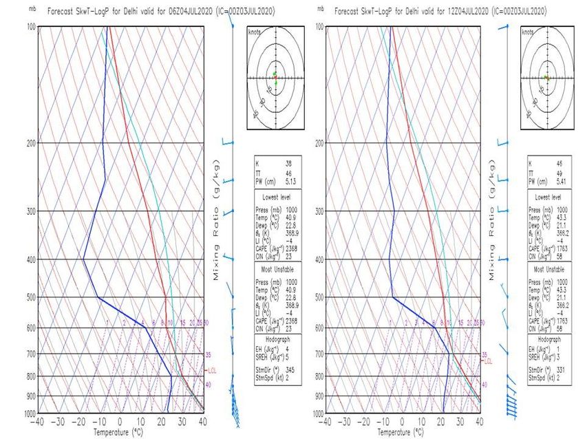
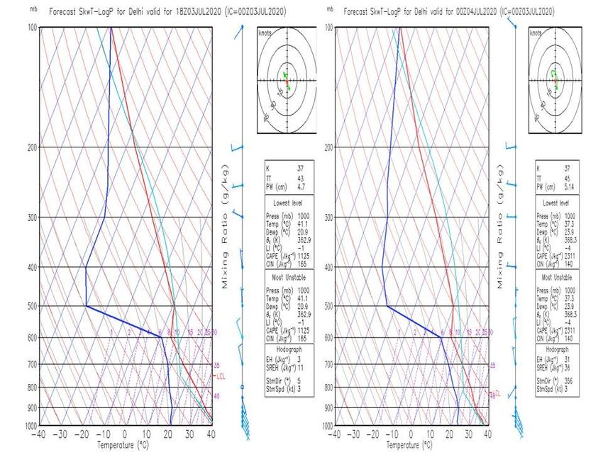
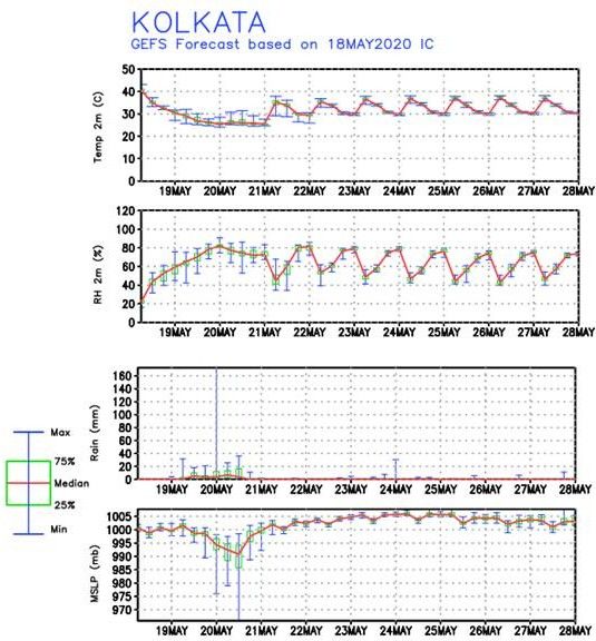
probability of having heavier category rainfall. It is worth to note that skillful prediction on block level
will eventually help to minimize the damage caused by the heavy and extreme rainfall events.

3.5 EPS Gram

 Figure 8 shows the EPS Meteogram (EPSgram) computed from the output of GEFST1534
based on 18th May initial condition over Kolkata. The EPSgram is a probabilistic interpretation of the
forecasts from the Ensemble Prediction System (EPS) for a given location. It displays the time
evolution of the distribution of atmospheric variables in the ensemble forecast. The red line
corresponds to the median of 20 member ensemble, i.e, it is showing the middle member of the upper
and lower half of the distribution. The top part of the blue bar is showing the maximum value of that
given variable amongst the 21 member ensemble and the lower part of it showing the minimum value
of the same variable. The lower line of the green box shows the value represented by the bottom 25%
of the members and the top line represents the value within which 75% of the members are laying. So
here we have chosen the EPSgrams from a recent cyclone AMPHAN that made the landfall on 20th
May 2020 over Sundarbans and eventually moved to Kolkata city and made massive destruction. The
figure shows that the 2m air temperature gradually decreases and becomes minimum between 20th to
21st May. After 21st it rises again. The rainfall also reaches maximum between 20th to 21st May and
decreases thereafter. It is to be noted that during the maximum rainfall the members are showing great
variation with the minimum value of no rain to a maximum value of more than 160 mmhr-1. It implies
that atleast one of the ensemble member indicates very heavy rainfall on 20th May over Kolkata.
Similar feature is also evident in the mean sea level pressure (MSLP) plot (bottom panel). MSLP
shows a minimum value during the same time as in the case of rainfall and 2m air temperature. Some
members even show MSLP as low as 970 mb. The EPSgram based on GEFS ensemble forecast
provide additional guidance over selected cities across India particularly during extreme events.

3.6 Skew-T plots

 Figure 9 shows the skew T-log P chart using GEFST1534 model forecast outputs based on
3rd July 2020 IC valid for 18, 24, 30 and 36 hours respectively over Delhi. This region was selected
because of monsoon onset on the national capital. The blue line represents the dew point
temperature of a parcel. Red line represents environmental temperature and cyan line represents the
temperature profile of a parcel lifted adiabatically from the surface. They are enclosed by the red
and cyan curve (enclosed by a black ellipse on the top right panel) represent CAPE. It is to be noted
that a cape value more than 1000 Jkg-1 is conducive for the development of thunderstorms. We have

 8

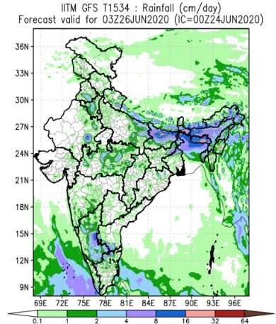
picked a thunderstorm case over Delhi on 4th July to show the evolution of skew T-log P charts. We
can see on 3rd July 18hrs the CAPE value increases to 1125 Jkg-1 but on 4th July 00 hrs it has
become almost double to 2311 Jkg-1. Figure 10 shows that the CAPE even further increases to 2368
Jkg-1 at 06hrs of the same day and then at 12 hrs it started reducing showing a value of 1763 Jkg-1.
The evolution of CAPE based on GEFS forecast thus demonstrates how this diagram can be very
useful to the forecasters to predict thunderstorm events in advance.

3.7 Probabilistic rainfall prediction over river basins for Flood Meteorological
Office (FMO)

 Increasing flood risk is recognized as one of the important threats in the changing climate
scenario especially in the perspective of extreme heavy rainfall events. In order to issue a warning
for flood, an appropriate quantitative precipitation forecast (QPF) system was required.
Probabilistic QPF (PQPF) providesthe best estimate of the chances that any given location will
receive an amount of rain that equals or exceeds a certain threshold value. In view of the above,
PQPF based on GEFS over different river basins has been operationalized recently. Twenty four
FMO (Flood Meteorological Office)/agencies those are responsible for issuing the QPF in the
respective regions. The said regions are Agra, Asansol, Ahmedabad, Bengaluru, Bengaluru-Kerala,
Bhubaneswar, Chennai, DVC, Guwahati, Hyderabad, Jalpaiguri, Lucknow, New Delhi, Patna,
Srinagar, Cauvery, Hirakud, Narmada, Krishna, Idamalayar, Idukki, Maithon, Tapi and Panchet.
GEFS based PQPF is produced daily for the above FMO basins in six different precipitation ranges
(viz. 0-0.1, 0.1-10, 10-25, 25-50, 50-100 and >100 mm).

Figure 11 shows (a)day-1, (b)day-3 and (c)day-5 PQPF forecast based on GEFS valid for 26 June
2020 over FMO Patna region which predicted a heavy rainfall, and created havoc/floods over the
region.There is more than 50% probability of rainfall between 10 to 25 mm with all the lead time
over the region. The model is also able to capture 25% probability of rainfall more than 100 mm
with 120hr lead time in few river catchments.PQPF forecasting is useful in issuing a flood warning
during monsoon season and extreme weather events.

4. Conclusions and Future works

 The GEFS model is ported on Pratyush and Mihir HPCS systems and has been in operational
mode from 01June 2018. The model is run twice (00UTC and 12UTC) a day with 10 days lead
 9

time. Various products are generated from this model for the forecasters. While it is demonstrated
in the above sections that ensemble prediction system based on GFS (GEFS) at the globally highest
resolution of 12.5 km is providing skillful predictions of a variety of weather systems with longer
lead time, there is a need to improve the fidelity of individual member in the ensemble and also
improve the performance of the GEFS system further. Mostly it is noted that the ensemble system
has a reasonable skill up to 5 days but for the disaster mitigation and early warning, there is a need
to extend the skill up to 7 days or beyond. Considering this societal need into account, the
GFS/GEFS system would be developed at a global 6 km resolution (over tropics) using cubic-
octahedral dynamical core. Along with the change of dynamical core, the future system would be
using Stochastic Physics Perturbation Tendencies (SPPT) in place of Stochastic Total Tendency
Perturbation (STTP). The present system uses 64 hybrid vertical levels which will be increased to
91 hybrid levels. The convection is currently being done using a scale-aware approach. The
convection and cloud microphysics would be further improved to incorporate the stochastic physics.
More data from remote sensing sensors and in-situ would be ingested to improve the initial
conditions.

5. Acknowledgement
 The support and encouragement by Director, IITM, Head, NCMRWF, DG, IMD and Secretary,
 MoES towards the implementation of the highest resolution GEFS system is gratefully
 acknowledged. MoES High Power Computing (HPC) facilities “Pratyush” located at IITM,
 Pune and “MIHIR” located at Noida and their support team are highly appreciated and
 acknowledged. National Centre for Environmental Prediction (NCEP), USA is acknowledged
 for sharing the latest version of GEFS and continuous support.

6. References

  Buizza R. and Palmer T.N., 1995: The singular vector structure of the atmospheric global
 circulation, Journal of the Atmospheric Sciences, 52, 1434-1456.
  Buizza R., Tribbia J., Molteni F., Palmer T.N., 1993: Computation of optimal unstable
 structures for a numerical weather prediction model, Tellus, 45A, 388-407.
  Buizza, R., Houtekamer, P. L., Toth, Z., Pellerin, P., Wei, M. and Zhu, Y.2005: A
 Comparison of
 the ECMWF, MSC and NCEP global ensemble prediction systems. Monthly Weather
 Review,133, 1076-1097.
  Leith C.E., 1965: Numerical simulations of the Earth‟s atmosphere. In: Alder B., Fernbach
 S., Rotenberg M., (Eds.) Methods in Computational Physics, New York, NY: Academic
 Press, pp. 1-28.
 10

 Liu H., Hu M., Stark D., Whitaker J., Shao H. and Newman K., 2015: Developmental
 Testbed Center, Ensemble Kalman Filter (EnKF) User's Guide for Version 1.0. Available at
 http://www.dtcenter.org/EnKF/users/docs/index.php.
 Lorentz E. N., 1963: Deterministic non-periodic flow, Journal of Atmospheric Science, 20,
 130-141.
 Mintz Y., 1965: Very long-term global integrations of the primitive equations of
 atmospheric motion, Proceedings of WMO/IUGG Symposium on Research and
 Development Aspects of Long-Range Forecasting, WMO Technical Note No 66, pp. 141-
 167
 Molteni F., Buizza R., Palmer T.N., Petroliagis T., 1996: The ECMWF ensemble prediction
 system: methodology and validation, Quarterly Journal of the Royal Meteorological Society,
 122, 73-119.
 Palmer T.N., Molteni F., Mureau R., Buizza R., Chapelet P., Tribbia J., 1992: Ensemble
 Prediction, ECMWF Technical Memorandum No. 188, Available at:
 https://www.ecmwf.int/en/elibrary/11560-ensemble-prediction
 RaghavendraAshrit, G.R. Iyengar, SyamSankar, Amit Ashish, AnumehaDube, Surya Kanti
 Dutta, V.S. Prasad, E.N. Rajagopal and Swati Basu,2012: Performance of Global Ensemble
 Forecast System (GEFS) During Monsoon, NCMRWF Report, NMRF/RR/1/2013.
 https://www.ncmrwf.gov.in/GEFS_Report_Final.pdf
 Smagorinsky J., 1963: General circulation experiments with the primitive equations,
 Monthly Weather Review, 92, 99-164.
 Toth Z., Kalnay E., 1993: Ensemble forecasting at NMC: the generation of perturbations,
 Bulletin of the American Meteorological Society, 74, 2317–2330.
 Toth Z., Kalnay E., 1997: Ensemble forecasting at NCEP and the breeding method, Monthly
 Weather Review, 125, 3297–3319.
 Wilks, D.S., 2011. Statistical methods in the atmospheric sciences (Vol. 100). Academic
 press.
 Zhu Yue Jian, 2005: Ensemble forecast: A new approach to uncertainty and predictability,
 Advances in Atmospheric Sciences, 22(6):781-788.

 11

Figure 1 Schematic view of the GEFS T1534 model

 18

 16

 14
 RMSE/Spread (mm/day)

 12

 10
 RMSE
 8
 Spread
 6

 4

 2

 0
 Day 1 Day 2 Day 3 Day 4 Day 5 Day 6 Day 7

Figure 2: RMSE and spread of precipitationforecast (mm day -1) over Indian landmass for JJAS
 of 2018 and 2019

 12

Figure 3: Brier Score and its decomposition of precipitationforecast (mm day -1) over Indian
landmass for JJAS of 2018 and 2019 for various thresholds with lead times.

 13

(a) (c)

 (b) (d)

Figure 4 a) INSAT 3D IR Brightness Temperature Image, (b) Mean Sea Level
Pressure from the analysis, (c) GEFS T1534 120 hr Forecast of Ensemble Mean and
Spread (shaded) for wind speed (vectors) at 850 hPa level and (d) Mean Sea Level
Pressure (contour) all valid for 00Z 20 JUNE 2020

 14

a c d e

 b f g h

 Figure 5. 24 hr accumulated rain from (a) IMD-GPM merged Gridded data, 48 hr forecast
 from (b) GFS and (c) GEFS ensemble mean along with the probability of rain with various
 thresholds (d) > 2.5 mm/day (e) > 15.6 mm/day, (f) > 65.5 mm/day, (g) > 115 mm/day and
 (h)195 mm/day or more all valid for 26th June 2020.

\
 15

(a) Strike Probability (c)

 (d)

 (b) Maximum Surface Wind

Figure 6. (a) Strike probability forecast, (b) Forecast of maximum surface wind speed
(knots) for Super Cyclone AMPHAN both based on 12Z 17MAY 2020 Initial Condition.
Here Black line (IMD) is from IMD best track data, blue line (AC00) is for the control run
and red lines are for the ensemble members with dark Red line (AEMN) for Ensemble
mean. Verification of the forecast of (c) track and (d) intensity from all the ICs during the
lifespan of the AMPHAN.

 16

Figure 7. Block level forecast of precipitation probability for different rainfall category (mmday-1)
valid for 20th May 2020 based on GEFS T1534 model forecast with 18th May 2020 IC. Different
blocks with corresponding districts names are mentioned. Orange (yellow) color indicates
precipitation probability more than 75% and yellow color represents probability 50%-75%. Aqua
color and sky-blue color represent probability (25%-50%) and (5%-25%) respectively.

 17

Figure 8.EPSgrams (Top panel to bottom panel ) of 2m temperature (oC), RH(%) at 2m,
Rain (mm/hr) and MSLP(mb) based on GEFST1534 outputs with 18th May 2020 initial
condition over Kolkata.

 18

Figure 9.Skew T-log P charts using GEFST1534 forecast products based on 3rd July 2020 initial
condition valid for 18hr,24hr respectively from the top left to bottom right panel over Delhi.

 19

Figure 10.Skew T-log P charts using GEFST1534 forecast products based on 3rd July
2020 initial condition valid for 30hr and 36 hr respectively from the top left to bottom
right panel over Delhi.

 20

(a)

 (b)

 (c)
 ))

Figure 11.QPF plot for the Patna river basin from the GEFS model on 26June 2020 for
a) one day lead b) three days lead and c) five days lead. The PQPF of more than 75
percentage is shown with 5 days lead.

 21