Macroscopic modeling of strain-rate dependent energy dissipation of superelastic SMAs considering destabilization of martensitic lattice - arXiv
←
→
Page content transcription
If your browser does not render page correctly, please read the page content below
Macroscopic modeling of strain-rate dependent
arXiv:2107.12145v1 [cond-mat.mtrl-sci] 16 Jul 2021

                                                     energy dissipation of superelastic SMAs considering
                                                     destabilization of martensitic lattice ‡
                                                                     A. Kaup, O. Altay and S. Klinkel
                                                                     Department of Civil Engineering, RWTH Aachen University,
                                                                     Mies-van-der-Rohe-Str. 1, 52074 Aachen, Germany
                                                                     E-mail: altay@lbb.rwth-aachen.de

                                                                     July 2019

                                                                     Abstract. Superelastic shape-memory alloys (SMAs) are unique smart materials
                                                                     with a considerable energy dissipation potential for dynamic loadings with varying
                                                                     strain-rates. The energy dissipation arises from a hysteretic phase transformation
                                                                     of the polycrystalline atomic grid structure. In fact, the nucleation from austenite
                                                                     to martensite phase and vice versa exhibits a strong thermomechanical coupling.
                                                                     The hysteresis depends on the latent heat generated by the austenitic-martensitic
                                                                     transformation and the convection of that heat. Due to the thermomechanical coupling,
                                                                     the martensitic nucleation stress level and thus the propagation of martensitic phase
                                                                     fronts strongly depends on the material temperature. High strain-rate interferes with
                                                                     the release of the latent heat to the environment and determines quantity, position and
                                                                     propagation of martensitic transformation bands. Lastly, high strain-rate reduces the
                                                                     hysteresis surface. The propagation velocity and quantity of martensitic bands have an
                                                                     impact on martensitic phase stability. The degree of atomic disorder and accordingly
                                                                     the change in entropy influences the reverse phase transformation from martensite
                                                                     to austenite. In other words, the stability of the martensitic state affects the stress
                                                                     level of the reverse transformation. However, in phenomenological superelastic SMA
                                                                     models, which are used to simulate energy dissipation behavior, the effects of the rate-
                                                                     dependent entropy change are not considered in particular.
                                                                         To incorporate the rate-dependent entropy change, we improved a one-dimensional
                                                                     numerical model by introducing an additional control variable in the free energy
                                                                     formulation for solid-solid phase transformation of superelastic SMAs. In this model,
                                                                     the observed effects of the strain-rate on the reverse transformation are taken into
                                                                     account by calculating the rate-dependent entropy change. A comparison of the
                                                                     numerical results with the experimental data shows that the model calculates the
                                                                     dynamic superelastic hysteresis of SMAs more accurately.

                                                     ‡ Accepted version of the paper published in Smart Materials and Structures, 29(2):025005, 2020, DOI:
                                                     10.1088/1361-665X/ab5e42
2
1. Introduction
Polycrystalline shape-memory alloys (SMAs) are applied in various fields in engineering.
SMAs with initial superelasticity are already extensively used in aeronautic, automotive
and healthcare engineering. Furthermore, interest in SMAs as a damper system
is growing in civil engineering [1]. In general, SMA-based engineering applications
experience predominantly strain-rate variated loadings. Especially in civil engineering
both seismic events and wind cause dynamic loading on structures. In order to
counteract this structural vibrations, several structural control strategies have been
developed. Commonly used damping systems, such as steel-hysteresis-dampers,
dissipate structural vibration energy by inelastic deformations. However, inelastic
damping devices cannot recover deformations and thus suffer loss of damping effects.
This problem motivates research into SMA-damping devices. In fact, superelastic
SMA-damping devices can reduce structural vibrations significantly without irreversible
deformations due to unique hysteretic behavior. The superelastic hysteretic material
behavior of SMA is thermomechanically triggered and includes both martensitic
transformation and reverse transformation. This study focuses on NiTi (Nickel
titanium) SMA wires, which are the most commonly used SMAs in damping systems.
For tensioned SMA wires, the stress level for phase transformation depends on strain-
rate and loading history. The loading history has a decisive impact on the hysteretic
behavior of NiTi wires if they are not trained. Accordingly, the in damping systems used
NiTi wires are trained and thus the loading history does not decrease the superelastic
hysteresis. Therefore, the loading history effects are not considered anymore in this
study. However, the strain-rate strongly influences the thermomechanically triggered
phase transformation. On the macroscopic level the nucleation from austenite to
martensite is composed by the formation of martensitic transformation bands.
The strain-rate dependent evolution of macroscopic transformation bands is
essential to consider strain-rate effects in constitutive modeling of superelastic SMAs.
One of the first investigations on the macroscopic formulation of phase transformation
fronts in NiTi was conducted by Shaw [2]. Another seminal study regarding both
the macroscopic and microscopic behavior of NiTi under cyclic loading was performed
by Otsuka [3]. Based on these investigations, Feng [4] used electromechanical-opting
testing machines and high resolution optical recorders to capture images of the material
surface during varying strain-rate loadings. Pieczyska [5], furthermore, used differential
scanning calorimetry (DSC) to record the thermal evolution of the macroscopic phase
transition bands, while additionally using infrared cameras to obtain thermograms.
Another method to investigate the stress induced martensitic transformation is to use
an acoustic emission sensor. In detail, Pieczyska [6] used an acoustic emission technique
to measure the propagation of stress waves, which are related to rapid local volume
changes. Precisely, in superelastic SMAs the evolution of martensitic transformation
bands triggers a change in the material volume and thus produces stress waves. By
comparing the acoustic emission to material temperature changes recorded by infrared3
camera and mechanical stress-strain diagrams it is possible to investigate the stress
induced nucleation and propagation of martensitic phase fronts. Amini [7, 8], conducted
nanoindentation tests on NiTi SMAs to investigate loading-rate dependent martensitic
nucleation and phase front velocity. Therefore, he used a nanonindenter to apply cyclic
loading, a 3D surface profiler to measure the surface roughness and DSC. Moreover,
Xiao [9] investigated the strain field and the temperature field of NiTi specimen with 3D
strain field cameras and infrared cameras. Also, Sun [10] used both speed and thermal
cameras to investigate the evolution and propagation of transformation domains for
varying stretching rates.
The strain-rate dependent constitutive modeling of superelastic SMAs for
civil engineering applications is predominantly formulated as macroscopic material
models. Brinson [11], Graesser [12] and Auricchio [13], among others, investigated
fundamental macroscopic models. In the last decades, researchers developed several
thermomechanical constitutive models for superelastic SMAs. In particular, Morin
et. al. [14] developed a three-dimensional constitutive model specialized for
thermomechanical coupling. A three dimensional finite element model focused on the
thermomechanical coupling in SMAs was also developed by Christ [15]. Moreover,
numerically simpler and thus computationally more efficient models were developed.
Ren [16] implemented a simple one-dimensional macroscopic model, which considers,
based on the Greasser model, the strain-rate effects on cyclic loaded SMAs using
the least square method. Furthermore, Zhu [17] developed a one-dimensional rate-
dependent model for tensile stress, using a Runge-Kutta integration scheme. Also,
Auricchio [18] developed a thermomechanical rate-dependent, one-dimensional model
based on his primary research. To cover the cycle-dependent behavior of superelastic
SMAs, Sameallah [19] proposes a further one-dimensional thermomechanical coupled
constitutive model. Cisse [20] proposes a review paper on modeling techniques for
superelastic SMAs. In general, all these models mainly differ in the free energy
formulation, the solution algorithm and the evolutionary equation. Besides, Yu’s [21]
one-dimensional model uses wave equations to cover the influence of the strain-rate on
the phase front velocity during martensitic transformation. Furthermore, Acar et al.
developed a numerical model based on neural networks and fuzzy logic, that covers
both the rate- and temperature dependent behavior of SMAs [22].
Both the evolution and propagation of martensitic phase fronts and the general
thermomechanical coupling strongly influence the thermal evolution and the hysteretic
behavior of dynamically excited SMAs. However, to our knowledge, simple and
thus numerically efficient one-dimensional constitutive models developed so far do
not explicitly consider the strain-rate dependent martensitic phase stability. In
particular, the stress induced martensitic phase stability depends on the phase band
nucleation and the velocity of phase front propagation. The quantity of martensitic
transformation fronts and the propagation velocity of these is influenced by the strain-
rate. Simultaneously, martensitic phase stability changes with the rate-dependent
evolution of transition fronts.4
This paper proposes an improved one-dimensional numerical model based on
Auricchio’s constitutive model [18], that allows integrating changes in phase stability
depending on the strain-rate. The chosen numerical model of Auricchio is suitable
for NiTi-wires as it is one-dimensional, and thus needs comparatively small number of
input parameters to calculate the hysteretic behavior of SMA dampers. Furthermore,
all the fundamental equations are thermomechanically consistent. The improved
model considers the destabilization of martensitic lattice with macroscopic modeling
approaches. Fast evolution of numerous phase bands, triggered by high strain-rate
loads, destabilizes the martensitic lattice. The proposed constitutive model includes the
energetic stability of the austenite phase state during increasing inherent temperature.
For this purpose, we introduce a free-energy formulation, which calculates the entropy
change in a strain-rate depending manner. The numerical model is validated by uniaxial
cyclic tensile tests applied on trained NiTi-SMA wires.
The paper is divided into four sections. Section 2 introduces the dynamic
material behavior of SMA and the experimental setup, which is used for the validation
of the numerical model. Subsequently, Section 3 presents the constitutive model
for superelastic SMA. Finally, the validation of the numerical calculations with the
experimental results is presented in Section 4.
2. PRELIMINARY
2.1. Dynamic material properties
The superelastic behavior of NiTi is thermomechanically coupled. For superelastic NiTi,
the austenitic grid structure is energetically more effective. Thus, energy, such as by
tensile stress, has to be applied to initiate a phase transition. Auricchio [18] defines in
detail, the stress-induced phase transformation as indicated by the critical martensitic
transformation start and finish points RsAM and RfAM and inversely by RsM A and RfM A .
Superscript AM indicates a transformation from austenite to martensite and M A vice
versa. To incorporate the thermomechanical coupling, the critical transition point R
depends on the stress level σ and the thermal level T . Indeed, the thermal level depends
on the entropy η, however, here entropy is not rate-dependent and thus only a constant
thermodynamic scaling factor.
R = σ − T (η) (1)
SMA’s thermal evolution depends on the latent heat generation during the exothermic
process, when the atomic grid restructures from a austenitic cubic to a martensitic
monoclinic grid. Indeed, both the latent heat generation and the convection of the
generated heat depend on the transformation-rate and on the diameter of the SMA
specimen. As a result, especially the critical transformation points RfAM and RsM A
shift upwards for a higher material temperature and consequently the slope of the
hysteretic transformation area increases. In general, for higher external temperatures the
whole hysteresis shifts upwards, because the high temperature austenite phase becomes5
martensite
strain direction
austenite
(a) (b)
Figure 1: Schematic martensitic transformation induced band evolution for quasi-static
(a) and dynamic (b) excitation. SMA wire fixed at both ends. Martensite-fractions are
illustrated as black transformation bands.
more stable and thus more stress is needed to initiate the phase transformation. This
phenomenon occurs regardless of the strain-rate and is considered by the Clausius-
Clapeyron coefficient [23]. However, the latent heat generation induces inherent
temperature changes, which influence the nucleation of the martensitic transformation
bands. Thus, both the external and the internal temperature have to be considered.
The phase transition induced thermal evolution is strain-rate and transformation-rate
dependent and has an essential influence on the hysteresis surface. Additionally, the
martensitic phase stability influences the reverse transformation. For instance, Fig. 1
illustrates the evolution of the martensitic transition fronts for both quasi-static (a) and
dynamic excitations (b). In a quasi-static load-state, the growth of localized martensite
bands determines the phase transition [9]. In general terms, for quasi-static excitation
the stress field specifies the position of the transition fronts; hence, they are located
next to the fixture points [2]. Evolution of the quasi-static martensite bands leads to
wider bands and comparative phase-stable martensitic modes. In contrast, a higher
strain-rate causes an increase of the nucleation sites in the material [7]. An increase in
the band quantity concurrently implies a decrease in the band width. Moreover, the
front propagation velocity rises corresponding the loading-rate. The evolution of several
coexistent transformation fronts destabilizes the intact structure of the material [2].
Consequently, the martensitic phase stability reduces for higher strain-rates, even if the
amount of the martensite-volume in the specimen is comparable to the quasi-static case.
In particular, the phase transition during high strain-rate loading induces an intrinsic
instability of the transformation domains [24]. The evolution of various both coexistent
and existent transition fronts and the evolution of new defect zones in the material,6
such as inclusions or dislocations, are mutually dependent [7]. In addition, the higher
transformation-rate raises the degree of atomic disorder and the motion of the atoms.
Indeed, a more unstable atomic state is concomitant with increasing entropy in the
material [25]. As a consequence, the reverse transformation process is initiated early on
a higher stress level, since the martensitic phase becomes too unstable and the material
strives for the energetically more efficient and more stable austenite grid structure.
It should be noted that the micromechanical processes during martensitic and reverse
transformations are nonsymmetrical [6]. Summarized, high strain-rates cause a decrease
of martensitic stability, which leads during unloading to a reverse transformation on the
higher stress level.
2.2. Experimental setup
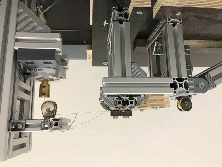
Fig. 2 shows the utilized shaking table for the uniaxial cyclic-tensile tests. The uniaxial
horizontal shaking table is 0.50 m x 0.50 m in size and can simulate both cyclic
and stochastic loadings. The major components of the experimental setup are the
shaking table (1) and a fixed test rig (2). NiTi wires (3) are attached to a vertically
installed load cell (4). The distance from load cell to the right-side fixture is 150 mm
and thus sets the NiTi wire length for the experimental investigations. The uniaxial
direction movement (5) causes tensile stress on the NiTi wire. To avoid buckling,
which is owing to pressure, a pulley (6) redirects the SMA-wire and ensure centric
load application to the load cell. Additionally, weights (7) pre-stress the NiTi wire to
induce martensitic transformation in a both faster and controlled manner. Moreover,
k
n
q
p
o l
m
j
Figure 2: Utilized experimental setup, side-view. (1) shaking table, (2) test rig, (3)
NiTi-wire, (4) load cell, (5), uniaxial strain direction, (6) pulley, (7) weights, (8) two
T-type thermocouples.7
two T-type thermocouples (8) are installed 5 and 60 mm distanced from the right-
side fixture. This position enables local temperature evolution measurement and the
identification of the local thermal differences. To control the table motion and to record
the measurements a MATLAB/Simulink environment is used. A CAN-hub connects the
MATLAB/Simulink code with the shaking table and introduces the excitation signals.
Finally, all sensors are connected with BNC-wires via a National Instruments NI USB-
6210 A/D converter to a PC.
3. Rate-dependent constitutive SMA model
In this section, an advanced macroscopic model is introduced, which accounts for the
entropy evolution to cover martensitic destabilization for high strain-rate tensile loads.
The model is based on the subsequently summarized model of Auricchio [18].
To cover the thermomechanical behavior of superelastic SMAs, the constitutive
model is based on thermodynamic potential state laws. To calculate the thermodynamic
material behavior we use a set of internal and external variables referring to a
homogenized volume element. In general, the internal variable ξ, representing the
martensitic volume fraction in the material, is expressed for martensitic transformation
in term of the following evolutionary equation
Ḟ
ξ˙ = β AM ξ 2 , (2)
F − RfAM
which can be controlled with the speed-parameter β AM . This equation depends
moreover on the driving force F and the thermo-coupled limit stress level for martensitic
transformation RfAM , where both depend on the external variables; the temperature T
and the uniaxial strain ε. To take into account the thermomechanical coupling, the
constitutive model is based on a formulation of the free energy ψ. In particular, the
derivation of ψ originates from the thermo-elastic free energy formulation for single-
phase materials of Raniecki and Bruhns [26] and reads
T
ψ = ψ0 (T ) + ψ e (εe ) − (T − T0 )η e (εe , T ) + C (T − T0 ) − T ln . (3)
T0
In this case, ψ0 states the temperature-dependent free energy connection to the
material’s internal energy u and entropy η in the reference state and ψ e states the
free energy dependency on elastic strain. Moreover, C is the material heat capacity and
T0 the reference temperature. The heat capacity C strongly influences the sensitivity of
the material to thermal changes. Based on Eq. 3, Auricchio and Sacco proposed a free
energy formulation [13] for solid-solid phase transformation in superelastic SMAs as,
T
ψ = [(uA − T ηA ) − ξ (∆u − T ∆η)] + C (T − T0 ) − T ln
T0
1 e2
+ Eε − (T − T0 ) εe Eα , (4)
2
where the subscript −A defines the austenite, ∆ the constant difference between
austenite and martensite values. Accordingly, ∆η is time-independent. Moreover, α8
is the thermal expansion and E the elastic modulus, which follows the Reuss-scheme.
The evolution of the elastic modulus depends on the martensitic volume ratio and thus
ranges from the austenitic elastic modulus and the martensitic elastic modulus. Based
on Eq. 4, the stress σ and the temperature T are defined by the corresponding derivations
of the free energy formulation. Hence, σ and T are defined, based on the heat equation
as
∂ψ
σ = e = Eεe − Eα (T − T0 ) (5)
∂ε
and
∂2ψ ∂2ψ ˙ ∂ψ ∂ψ ˙
C Ṫ = T e
ε̇ + T ξ + σ ε̇ − ε̇ − ξ − γ (T − Text ) . (6)
∂T ∂ε ∂T ∂ξ ∂ε ∂ξ
To incorporate the rate-dependent entropy change, we rewrite ψ0 (T ), part of the free
energy formulation of Eq. 3, by introducing the time-dependent entropy difference ∆η(t)
to define ψ as
T
ψ = [(uA − T ηA ) − ξ (∆u − T ∆η(t))] + C (T − T0 ) − T ln
T0
1 2
+ Eεe − (T − T0 ) εe Eα . (7)
2
More in detail, ηA states for t = 0 the entropy level of the material in the pure austenite
state. This state is also reached after each complete relief of strain and thus after each
completed reverse transformation. Since we deal with thin wires, we neglect the thermal
expansion factor α subsequently. Now, we introduce
∂ψ T
η(t) = − = ηA + ξ∆η(t) + C ln , (8)
∂T T0
which updates η not only depending on ξ and T but also on ∆η(t) with
∆η(t) = η(t) − ηA , (9)
as an additional control variable, which defines the difference between the current
entropy level η(t) and the initial entropy level ηA and thus considers a time-dependent
and strain-rate dependent calculation of the entropy change. The rate-dependent
entropy change calculation enables to consider the strain-rate effects on the reverse
transformation. The increasing entropy is the measure to define the strain-rate
dependent instability of the martensitic state. The rate-dependency of the calculation
arises directly from ξ, which depends on the phase transformation-rate, and from T . In
fact, the rate-dependency of T comes directly from ε̇ and ξ˙ in Eq. 6. At this point, it is
important to note, that with the existing temperature equation of the primary model the
calculated evolution of the simulation temperature T is only qualitatively comparable
to the experimentally measurable real temperature TE . Experimental results show that
the temperature increase is overestimated particularly for quasi-static excitations. In
order to counteract this overestimation, we introduce the scaling factor κ, which reduces
the temperature influence in the entropy calculation for the quasi-static load case. The
differentiation between quasi-static and dynamic load cases depends on the entropy9
evolution. In detail, ηqs is a threshold, which must be exceeded to calculate η following
Eq. 8. For quasi-static load cases, when η < ηqs , this paper proposes the entropy
calculation dependent on κ as follows,
∂ψ T
η(t) = − = ηA + ξ∆η(t) + κC ln ; f or η < ηqs (10)
∂T T0
Further research on the temperature equation is required to make the scaling factor κ
dispensable for future works. Nevertheless, the consideration of the rate-dependent
entropy change enables already the inclusion of the influence of martensitic phase
stability in the calculation. To consider the strain-rate effects, both on the initial
and final reverse transition stress level and on the martensitic-austenitic hysteresis
slope, we reformulate the thermo-coupled initial and final stress levels for the reverse
transformation and the corresponding speed parameter as
MA MA η(t)
Rs,f = σs,f − TR , (11)
εL
and
η(t)
βMA = . (12)
ηA
The reformulation of the thermo-coupled reverse transformation stress levels comprises
the strain-rate dependent entropy. Thus, the initial and final stress levels change by
altering the entropy level depending on the strain-rate. The thermo-coupled initial stress
level RsM A determines the initial reverse transformation strain εM A
s (η) and thus also the
linear-elastic part of the austenitic-martensitic phase transition. More in detail, this
material model is strain-driven and consequently we need strain values, which indicate
the begin and finish of the reverse transformation. These strain levels are updated
in every calculation step and thus change with varying entropy level to consider the
martensitic instability for high strain-rates. Consideration of the entropy change for
the initial and reverse strain levels of the austenitic transition leads to an increase of
εM A MA
s (η) and a decrease of εf (η) with increasing strain-rate. Next, the speed parameter
β M A (η) increases with increasing strain-rate and thus the reverse transformation slope
changes from a convex to a concave slope. In brief, the free energy reformulation enables
a rate-dependent calculation of the entropy change and hence the introduction of both
the entropy dependent speed parameter β M A (η) and the entropy dependent reverse
transformation strains εM A
s,f (η).
4. Results and discussion
The following part will discuss both experimental and numerical results, by which the
presented one-dimensional model will be validated. The experimental results in Fig. 3
visualize the strain-rate effects during cyclic-tensile excitation with a strain amplitude
of 4 % on trained 0.2 mm diameter Ni-55.8%-Ti-43.55%-SMA-wires, produced by SAES
Getters S.p.A. (SAES). In fact, we focus on the first loading cycle of each cyclic tensile
test. Since we deal only with trained wires the hysteresis can be assumed not to change10
anymore for increasing amounts of load cycles itself. We choose still the first load
cycle to be sure that every presented experimental result starts with the same initial
temperature, without former self-heating due to cyclic loading. While comparing the
whole hysteresis surface for frequencies of 0.05, 0.1, 0.5, 1.0 and 2.0 Hz, we visualize both
the linear-elastic and the transformation section of the reverse transition. We observe an
increase in the reverse phase transformation stress level and especially an upward shift in
transformation plateau with increasing slope corresponding to the increasing strain-rate.
As shown in previous studies, such as in [27, 28], the significance of the effect changes
depending on the thermodynamic properties of the SMA. In the results of Fig. 3, the
chosen wire geometry and loading configuration magnifies the reverse transformation
shift allowing us to show the entropy effect more clearly. The reverse transformation
MA
stress levels σs,f increase for increasing strain-rate. However, for high-strain rate tests,
the exact position of the reverse transformation finish level cannot be observed clearly
anymore, due to the direct phase transition of the investigated wires. Moreover, the
decrease of the linear-elastic reverse transformation for increasing strain-rates becomes
evident, as marked with a solid line in the plots. The decreasing linear-elastic section and
the resulting reverse transformation on a higher stress level strongly influence the shape
of the reverse transition hysteresis. The earlier the reverse transformation is initiated,
the more directly the austenitic phase transition takes place. Concurrently, the fast
and direct austenitic nucleation under high strain-rates causes a change of the reverse
hysteresis slope. In particular, the slope changes from a convex Fig. 3(a) to a straight
concave slope Fig. 3(e). This strain-rate dependent reverse transition shape is triggered
by the decreasing martensitic phase-stability. The decreasing martensitic phase stability
intensifies the strive to the energetically more effective austenite state. However, to our
knowledge, the existing constitutive models do not consider these strain-rate dependent
changes in the reverse transformation.
Subsequently, we present the effect of the entropy-change dependent calculation
step by step, both of the reverse transformation strains εM A
s,f (η) and the adjusted speed
parameter β M A . More precisely, the results are presented in the following order: no
rate-dependent entropy change, entropy change adjustment of εM A
s (η), entropy-change
adjustment of εM A
s,f (η) and β
MA
(η).
The performed numerical calculations use a set of material and thermodynamic
parameters. Because of its thermodynamic consistency, the material model can
be used beside wires also for uniaxially stressed bars and cables by tuning the
material and thermodynamic parameters of the model as listed in Table 1. We
selected the material parameters, apart from the thermodynamic parameters, on the
basis of quasi-static tensile tests taken both from the SAES data-sheet and self-
conducted experimental results. The thermodynamic parameters were not determined
experimentally, but chosen based on previous studies [18]. Accordingly, we chose the
following thermodynamic parameters appropriately to the behavior of the constitutive
model in a physically consistent manner, see Table 1. The material parameter εL is
the maximum residual strain, γ is a heat convection coefficient and Text and TR are11
350 350 350 350 350
300 300 300 300 300
250 250 250 250 250
200 200 200 200 200
150 150 150 150 150
100 100 100 100 100
50 50 50 50 50
0 0 0 0 0
0 1 2 3 4 0 1 2 3 4 0 1 2 3 4 0 1 2 3 4 0 1 2 3 4
(a) (b) (c) (d) (e)
Figure 3: Cyclic-tensile-tests on Ni-55.8%-Ti-43.55%-SMA wires. Red-marked solid
line: martensitic linear-elastic section. Dashed line: reverse transformation. Strain
amplitude: ε = 4 %. Excitation frequency: f = 0.05(a)/0.1(b)/0.5(c)/1.0(d)/2.0(e) Hz.
Wire length: L = 150 mm. Wire diameter: d = 0.2 mm. Pre-stress: σ0 = 134.9 MPa.
Ambient temperature: T = 22.5 ◦ C.
the external and the reference temperatures, respectively. The chosen thermodynamic
parameters are in a similar range of values as in literature, such as in [18]. ∆u and
∆η are used for the introduced entropy calculation and therefore differ from previous
studies.
To show the influence of the rate-dependent entropy change on εM A
s (η), we first
compare the numerical results, excluding the entropy calculation, with the experimental
results, see Fig. 4. The linear-elastic part of the calculation is again separately
marked. Indeed, the calculation of the martensitic-transformation is highly plausible
for the three frequencies of 0.05, 0.1 and 0.5 Hz. Although the rate-dependent
evolution of the simulation equals only qualitatively to the experimental temperature
TE , the model can represent the thermomechanical coupling for austenitic-martensitic
transition. However, the linear-elastic reverse-transformation section does not change
and the reverse transformation shape remains nearly the same. As a result, the hysteresis
area for high strain-rate excitation is overestimated. Furthermore, the deviations in the
calculation of the reverse transformation become evident.
For increasing strain-rates the difference between experimental and the numerical
reverse transformation finish stress level increases continuously. Next, Fig. 5, shows
the included entropy-change effect on εM A
s (η). To illustrate the effects of the entropy
change on εM A
s (η), we compare Fig. 5 with Fig. 4 and conclude that the linear-elastic
section decreases for increasing strain-rate, when entropy-change effects are included in
the numerical model. Nevertheless, the reverse transformation shape remains nearly12
Table 1: Material and thermodynamic parameters used for the constitutive model
Parameter Value Unit
EA 32350 MPa
EM 18550 MPa
εL 3.34 %
σsAM 85 MPa
σfAM 305 MPa
σsMA 225 MPa
σfMA 200 MPa
∆u 1320 MPa
ηA 0.0093 MPaK−1
ηqs 1.3 ηA MPaK−1
κ 0.0035 -
γ 0.1 -
C 4.0 MPaK−1
Tu 573 K
Text = T0 = TR 295.65 K
α 0 K−1
the same, even though the phase transition is introduced at a higher stress level.
The red-marked linear elastic section marks the calculated area between the beginning
of unloading condition and the beginning of the reverse transformation calculation.
Actually, significant changes in the reverse transformation arise firstly after activating
both the entropy dependent speed parameter β(η) and the reverse transformation finish
strain εM A
f (η). Accordingly, further entropy dependent adjustments are necessary for a
more accurate calculation of martensitic phase stability.
To incorporate the change in reverse transformation curve, we introduce the
rewritten speed parameter β M A as a function of η. In fact, β M A (η) defines the shape
of the cubic evolutionary equation for the reverse transformation and increases with
increasing entropy, see Eq. 12. Fig. 6 shows the numerical results both including and
excluding entropy changes, and compares the numerical to the experimental results.
Here, εM A
s,f (η) and β
MA
(η) are included in the calculation. The linear elastic area
decreases for increasing entropy by way of updating εM A
s (η). Simultaneously, the
reverse transformation finish stress decreases for increasing entropy, since εM A
f (η) is
included in the calculation. Last, the speed parameter β M A (η) increases for increasing
entropy and thus effectuates a reverse transformation slope change. Precisely, for quasi-
static excitation in Fig. 6(a) the numerical results with both excluded and included
entropy change have a convex reverse transition slope and can represent the experimental
results plausible. For a frequency of 0.1 Hz the experimental results already reveal a
decrease of the linear-elastic section and thus a steeper reverse transition slope, Fig. 6(b).
Comparing the numerical results of Fig. 6(b), we see the importance of εM A
s (η). Besides,
the change from a convex to an almost straight reverse transformation curve, we can
also observe an earlier initiation of the reverse transition. Indeed, the prior initiation13
350 350 350
300 300 300
250 250 250
200 200 200
150 150 150
100 100 100
50 50 50
0 0 0
0 1 2 3 4 0 1 2 3 4 0 1 2 3 4
(a) (b) (c)
Figure 4: Comparison of experimental data with numerical results excluding entropy-
change effects. Red-marked solid line: martensitic linear-elastic section. ε = 4 %.
f = 0.05(a)/0.1(b)/0.5(c) Hz. L = 150 mm. d = 0.2 mm. σ0 = 134.9 MPa.
T = 22.5 ◦ C.
350 350 350
300 300 300
250 250 250
200 200 200
150 150 150
100 100 100
50 50 50
0 0 0
0 1 2 3 4 0 1 2 3 4 0 1 2 3 4
(a) (b) (c)
Figure 5: Comparison of experimental data with numerical results including entropy-
change effects on εM A
s (η). Red-marked solid line: martensitic linear-elastic section.
ε = 4 %. f = 0.05(a)/0.1(b)/0.5(c) Hz. L = 150 mm. d = 0.2 mm. σ0 = 134.9 MPa.
T = 22.5 ◦ C.
arises from the entropy dependent calculation of εM A
s (η), while the change of the slope
comes from β M A (η). Even with the slight frequency increase from 0.05 to 0.1 Hz, the14
350 350 350 350 350
300 300 300 300 300
250 250 250 250 250
200 200 200 200 200
150 150 150 150 150
100 100 100 100 100
50 50 50 50 50
0 0 0 0 0
0 1 2 3 4 0 1 2 3 4 0 1 2 3 4 0 1 2 3 4 0 1 2 3 4
(a) (b) (c) (d) (e)
Figure 6: Comparison of experimental data with numerical results both excluding and
including entropy change. Thin solid line (blue): experimental investigation. Thick
solid line (black): numerical results; including entropy change. Dotted line: numerical
results; excluding entropy change. Entropy-change effects on εM A
s,f (η) and β
MA
(η).
ε = 4 %. f = 0.05(a)/0.1(b)/0.5(c)/1.0(d)/2.0(e) Hz. L = 150 mm. d = 0.2 mm.
σ0 = 134.9 MPa. T = 22.5 ◦ C.
overestimation of the hysteresis surface can happen but can be reduced by including
entropy changes in the calculation. In addition to the previously mentioned advantages
of the included entropy changes, we now focus on the high strain-rate results in Fig. 6
(c), (d) and (e) and the influence of εM A
f (η). All three results for high strain-rates are
appropriate to illustrate the difference between εM f
A
and εM A
f (η). Comparing the finish
reverse transformation stress σfM A of both numerical results for a frequency of 0.5 Hz,
we observe a difference of more than 50 MPa. In particular, by excluding the entropy
change, the numerical model overestimates the experimental σfM A and, moreover, the
phase transition to the linear-elastic austenitic part becomes abrupt. This abrupt
transition does not fit to the experimental results. However, the numerical model with
including entropy change effect calculates σfM A fairly well and thus also allows a smooth
transition from the phase transition to the linear-elastic austenitic section. In conclusion,
the inclusion of the rate-dependent entropy change for the reverse transition improves
the calculation accuracy. Furthermore, the austenite transformation changes for higher
strain-rate from a convex to a slightly concave curve due to the entropy dependent
calculation of β M A (η). Moreover, the initial (finish) level for reverse transformation
rises (decreases) for increasing strain-rates. Consequently, the advancements on the
one-dimensional material model enable, especially for high strain-rates, a more accurate
calculation of the hysteresis surface without negative impact on the numerical efficiency
of the algorithm, which both will be proved numerically in the following.15
Figure 7: Dissipated energy per load cycle. Comparison of experimental data with
numerical results both excluding and including entropy change. ε = 4 %. f =
0.05/0.1/0.5/1.0/2.0 Hz. L = 150 mm. d = 0.2 mm. σ0 = 134.9 MPa. T = 22.5 ◦ C.
To illustrate the improvement of the numerical model, Fig. 7 visualizes the
dissipated energy ED in [Nmm] of one load cycle for frequencies of 0.05, 0.1, 0.5, 1.0
and 2.0 Hz. For each frequency we compare the dissipated energy of the experimental
data with numerical results with both excluded and included entropy changes in the
calculation. The dissipated energy corresponds to the hysteresis surface calculated from
the force-displacement curve. In general, Fig. 7 shows, for all previously in Fig. 6 shown
three results, the decreasing energy dissipation of the superelastic SMA for an increasing
strain-rate. Furthermore, these results reveal a significant difference of the dissipated
energy between the quasi-static case with f = 0.05 Hz and the dynamic case with f ≥ 0.5
Hz. The accuracy difference of both calculation does not change for the dynamic cases.
Taking into account the quasi-static case, both numerical models slightly underestimate
the energy dissipation of the experimental results. However, for increasing strain-rate the
numerical results with excluded entropy-change effects always overestimate the energy
dissipation compared to the experimental results. In fact, the difference continues to
increase with increasing strain-rate. In contrast, the dissipated energy of the numerical
calculation, with considered entropy effects, decreases analogously to the experimental
results. Even though the entropy change included model slightly underestimates the
energy potential compared to the experimental results, the results differ significantly
less. Accordingly, the numerical model with including entropy change effects calculates
the hysteresis surface more accurately than the comparative model and thus conforms
with the experimental data.16
1.80
1.31
1.13
0.93
0 2 4 6 8 10
(a) (b)
25 4
3.5
24.5
3
2.5
24
2
23.5
1.5
1
23
0.5
22.5 0
0 2 4 6 8 10 0 2 4 6 8 10
(c) (d)
Figure 8: Comparison of (a) numerical entropy calculation; (b) simulation temperature
evolution; (c) experimental temperature evolution TE ; (d) strain-time history. ε = 4 %.
f = 0.05(a)/0.1(b)/0.5(c) Hz. L = 150 mm. d = 0.2 mm. σ0 = 134.9 MPa.
T = 22.5 ◦ C.
Next, we concentrate on the calculation time of the numerical models. The
calculation time using a standard PC differs between the two numerical models for
one load cycle with 2 Hz in average 0.006 seconds, which is negligibly small.
After discussing the numerical and experimental results concerning the hysteresis
surface and damping capacity, we will subsequently deal with entropy- and temperature
evolution per se. For this purpose, the numerical entropy- and the simulation
temperature evolutions are shown in Fig. 8 (a) and (b). The experimental temperature
results are illustrated in Fig. 8 (c) and the related strain curves in Fig. 8 (d). Each
subdiagram illustrates the evolution for one load cycle with a frequency of 0.05,
0.1 and 0.5 Hz. The temperature and the entropy increases for increasing strain-
rate. As mentioned prior, the calculated simulation temperature T is not equal
to the experimentally measured temperature TE . For the entropy-change dependent17 calculation, the slope and the course of the simulation temperature are still decisive, therefore, Fig. 8 (b) does not include any specific values. This diagram is intended to illustrate that the simulation temperature evolution corresponds approximately to the measured experimental temperature development and, moreover, the diagram has the purpose to demonstrate the influence of the temperature behavior on the numerical entropy evolution. Even though the entropy evolution (a) and the simulation temperature evolution (b) are quite similar, they differ explicitly in the start and finish values. Considering one completed load cycle, the entropy will always start and finish at ηA , because as soon as the material is completely in its austenite shape again, there is no increase in entropy due to the martensitic instability anymore. More in detail, at zero-stress level and an ambient temperature over the critical austenite finish temperature, the SMA is always in the superelastic state, where the austenitic grid- structure is energetically more efficient. In this state, the initial entropy condition ηA always applies. A stress induced phase transformation leads to an increased entropy evolution during loading. The simulation temperature, on the other hand, will initially start at Tref , but, depending on the excitation, the temperature at the end of one load cycle can be both higher or lower compared to the initial temperature. Thus, for the next load cycle the temperature calculation will start on the appropriate temperature level, while the entropy calculation will start at ηA again. Last, the experimental temperature data (c) results from the T-type thermocouple installed 60 mm distanced from the right-side fixture. The graph is shifted to the room temperature of T = 22.5 ◦ C as initial temperature. Although, the wire is only 0.2 mm in diameter the temperature increases for one load cycle with 0.5 Hz and a strain amplitude of 4 % more then 2 ◦ C. In summary, the temperature curve can be qualitatively calculated with the numerical model and further the comparison of the subdiagrams in Fig. 8 verifies the plausibility of the simulation temperature and the entropy evolution. 5. Conclusions In this paper, the influence of the rate-dependent phase-stability during the martensitic transformation of superelastic SMA-wires on the hysteresis surface is investigated both experimentally and considered numerically. To consider the rate-dependent phase- stability numerically, we advanced a one-dimensional macroscopic model by introducing an improved free energy formulation for the phase transition of superelastic SMA- wires. The proposed free energy formulation enables the rate-dependent entropy change calculation in the material to consider the decreasing martensitic phase- stability for increasing strain-rates. In brief, the entropy change calculation enables a strain-rate dependent calculation of the initial and finish strain level for the reverse transformation. The advancement further influences the reverse evolutionary equation and thus the shape of martensitic-austenitic transformation. Hence, the change from a convex to a concave reverse transition shape for increasing strain-rates can be calculated more accurately. The significant influence of the strain-rate on the
18

reverse transformation is shown by experimental results. In particular, we performed
cyclic-tensile tests with varying strain-rates on NiTi-wires, using a uniaxial horizontal
shaking table. Furthermore, the fundamental findings of the previous research on the
evolution of martensite transformation bands are gathered. Thus, both the relationship
between strain-rate and martensitic phase stability and the necessity for a numerical
consideration of this relationship have been noted. Furthermore, the experimental
results are utilized to validate the improved one-dimensional model. Besides the
comparison of the hysteresis surface of the numerical and the experimental stress-strain
diagrams, we also compared the experimental and the simulation temperature evolution
to determine the plausibility of the calculated entropy evolution. In conclusion, the
rate-dependent thermomechanical modeling of the entropy changes in superelastic SMAs
enables to consider the martensitic phase stability effects on the reverse transformation.
This allows a more accurate calculation of the hysteresis surface, as shown in this paper
by the presented calculations and experiments, with neither impairment of the numerical
models simplicity nor the robustness of the solution algorithm.
     The key features of the presented work are:
  • a free energy formulation incorporating the rate-dependent entropy change
  • consideration of strain-rate dependent martensitic phase stability in an one-
    dimensional macroscopic model
  • introduction of an entropy-dependent speed-parameter β M A (η)

Acknowledgments

The authors would like to express their sincere appreciation for the financial support
from the German Research Foundation (Deutsche Forschungsgemeinschaft, DFG) with
the grant number: KL 1345/12-1.

References

 [1] Fang, C. and Wang, W. 2019 Shape memory alloys for seismic resilience. (Springer)
 [2] Shaw, J. A. and Kyriakides, S. On the nucleation and propagation of phase transformation fronts
       in a NiTi alloy. Acta Mater. (1997) 45:683-700
 [3] Miyazaki, S., Imai, T. and Otsuka, K. Effect of cyclic deformation on the pseudoelasticity
       characteristics of Ti-Ni alloys. Int. J. Solids Struct. (1986) 38:6123-6145
 [4] Feng, P. and Sun, Q. P. Experimental investigation on macroscopic domain formation and evolution
       in polycrystalline NiTi microtubing under mechanical. J. Mech. Phys. Solids (2006) 54:1568-
       1603
 [5] Pieczyska, E. A., Tobusji, H. and Kualasinski, K. Development of transformation bands in TiNi
       SMA for various stress and strain rates studied by a fast and sensitive infrared camera. Smart
       Mater. (2013) 22:035007
 [6] Pieczyska, E. A., et.al. Martensite transformation bands studied in TiNi shape memory alloy by
       infrared and acoustic emission techniques. Kovove Mater. (2012) 50:309-318
 [7] Amini, A., Cheng, C. and Asgari, A. Combinational rate effects on the performance of nano-grained
       pseudoelastic Nitinols. Mater. Lett. (2013) 105:98-101
19
[8] Amini, A., Cheng, C., Kan, Q. Naebe, M. and Song, H. Phase transformation evolution in NiTi
shape memory alloy under cyclic nanoindentation loadings at dissimilar rates. Scientific Reports
(2013) 3:3412-3419
[9] Xiao, Y., Liu, Y. and Novak, V. On the origin of Lüders-like deformation of NiTi shape memory
alloys. J. Mater. Eng. Perf. (2015) 24:3755-3760
[10] Sun, Q. P., Zhao, H., Zhou, R., Saletti, D. and Yin, H. Recent advances in spatiotemporal evolution
of thermomechanical fields during the solid–solid phase transition. C. R. Méc. (2012) 340:349-
358
[11] Brinson, L. C., One-dimensional constitutive behaviour of shape memory alloys: Thermomechan-
ical derivation with non-constant material functions and redefined martensite internal variable.
J. Intell. Mater. Syst. Struct. (1993) 4:229-242
[12] Graesser, E.J. and Cozzarelli, F.A. Shape-memory alloys as new materials for aseismic isolation.
J. Eng. Mech. (1991) 117:2590-2608
[13] Auricchio, F. and Sacco, E. A one-dimensional model for superelastic shape-memory alloys with
different elastic properties between austenite and martensite. Int. J. Non Linear Mech (1996)
32:1101-1114
[14] Morin, C., Moumni, Z. and Zaki, W. A constitutive model for shape memory alloys accounting for
thermomechanical coupling. Int. J. Plast. (2011) 27:748-767
[15] Christ, D. and Reese, S. A finite element model for shape memory alloys considering
thermomechanical couplings at large strains. Int. J. Solids Struct. (2009) 46:3694-3709
[16] Ren, W., Li, H. and Song, G. A one-dimensional strain-rate-dependent constitutive model for
superelastic shape memory alloys Smart Mater. Struct. (2007) 16:191-197
[17] Zhu, S. and Zhang, Y. A thermomechanical constitutive model for superelastic SMA wire with
strain-rate dependence. Smart. Mater. Struct. (2007) 16:1696-1707
[18] Auricchio, F. and Sacco, E. Thermo-mechanical modeling of a superelastic shape-memory wire
under cyclic stretching-bending loadings. Int. J. Solids Struct. (2001) 38:6123-6145
[19] Sameallah, S., Kadkhodaei, M., Legrand, V., Saint-Sulpice, L. and Chirani, S. A. Direct numerical
determination of stabilized dissipated energy of shape memory alloys under cyclic tensile
loadings. J. Intell. Mater. Syst. Struct. (2015) 26:2137-2150
[20] Cisse, C., Zaki, W. and Zineb, T.B. A review of modeling techniques for advanced effects in shape
memory alloy behavior. Smart Mater. Struct. (2016) 25:103001
[21] Yu, H. and Young, L. M. One-dimensional thermomechanical model for high strain-rate
deformation of austenitic shape memory alloys. J. Alloy Comp. (2017) 710:858-868
[22] Acar, E., Ozbulut, O. E. and Karaca, H. E. Experimental investigation and the modeling of
the loading rate and temperature dependent superelastic response of a high-performance shape
memory alloy. Smart Mater. Struct. (2015) 24:075020
[23] Casciati, S., Faravelli, L. and Vece, M. Long-time storage effects on shape memory alloy wires.
Acta. Mech. (2018) 229:697-705
[24] He, Y. J. and Sun, Q. P. Rate-dependent domain spacing in a stretched NiTi strip. Int. J. Solids
Struct. (2010) 47:2775-2783
[25] Tatar, C. and Yildirim, Z. Phase transformation kinetics and microstructure of NiTi shape memory
alloy: Effect of hydrostatic pressure. Bull. Mater. Sci. (2017) 40:799-803
[26] Raniecki, B. and Bruhns, O. Thermodynamic reference model for elasto plastic solids undergoing
phase transitions. Arch. o. Mech. (1991) 43:343-376
[27] Zhang, X., Feng, P., He, Y. J., Yu, T. and Sun, Q. P. et.al. Experimental study on rate dependence
of macroscopic domain and stress hysteresis in NiTi shape memory alloy strips. Int. J. Solids
Struct. (2010) 52:1660-1670
[28] Zhang, Y., Zhu, J., Moumni, Z., Van Herpen, A. and Zhang, W. Energy-based fatigue model
for shape memory alloys including thermomechanical coupling. Smart. Mater. Struct. (2016)
25:35-42You can also read