INDIAN JOURNAL OF SCIENCE AND TECHNOLOGY - AWS
←
→
Page content transcription
If your browser does not render page correctly, please read the page content below
INDIAN JOURNAL OF SCIENCE AND TECHNOLOGY

RESEARCH ARTICLE

                                       Prediction of IPL matches using Machine
                                       Learning while tackling ambiguity in
                                       results
     OPEN ACCESS                       Ayush Tripathi1 ∗ , Rashidul Islam2 , Vatsal Khandor3 ,

Received: 12.09.2020
                                       Vijayabharathi Murugan4
Accepted: 17.10.2020                   1 Department of Computer Science, Raj Kumar Goel Institute of Technology, Ghaziabad,
                                       Tel.: +91-95-6010-4441
Published: 28.10.2020
                                       2 Department of AEIE, Heritage Institute of Technology, Kolkata, India
                                       3 Department of Computer Engineering, Dwarkadas J. Sanghvi College of Engineering,
Editor: Dr. Natarajan Gajendran        Mumbai
                                       4 Department of Chemical Engineering, Indian Institute of Technology, Madras
Citation: Tripathi A, Islam R,
Khandor V, Murugan V (2020)
Prediction of IPL matches using
Machine Learning while tackling        Abstract
ambiguity in results. Indian Journal
of Science and Technology 13(38):      Background/Objectives: The IPL (Indian Premier League) is one of the most
4013-4035. https://doi.org/            viewed cricket matches in the world. With a perpetual increase in the popularity
10.17485/IJST/v13i38.1649
                                       and advertising associated with it, forecasting the IPL matches is becoming
∗
    Corresponding author.              a need for the advertisers and the sponsors. This paper is centered on
Tel: +91-95-6010-4441                  the implementation of machine learning to foretell the winner of an IPL
ayushtr0904@gmail.com                  match. Methods/Statistical analysis: The cricket in the T-20 format is highly
Funding: None                          unpredictable - many features contribute to the result of a cricket match, and
Competing Interests: None
                                       each attribute feature has a weighted impact on the outcome of a game.
                                       In this paper, first, a meaningful dataset through data mining was defined;
Copyright: © 2020 Tripathi et al.
This is an open access article         next, essential features using various methods like feature engineering and
distributed under the terms of the     Analytic Hierarchy Process were derived. Besides, a key issue on data symmetry
Creative Commons Attribution
                                       and the inability of models to handle it was identified, which extends to
License, which permits unrestricted
use, distribution, and reproduction    all types of classification models that compare two or more classes using
in any medium, provided the            similar features for both the classes. This concept in the paper is termed as
original author and source are
                                       model ambiguity that occurs due to the model’s asymmetric nature. Alongside,
credited.
                                       different machine learning classification algorithms like Naïve Bayes, SVM, k-
Published By Indian Society for
                                       Nearest Neighbor, Random Forest, Logistic Regression, ExtraTreesClassifier,
Education and Environment (iSee)
                                       XGBoost were adopted to train the models for predicting the winner. Findings:
ISSN
                                       As per the investigation, tree-based classifiers provided better results with
Print: 0974-6846
Electronic: 0974-5645                  the derived model. The highest accuracy of 60.043% with Random Forest,
                                       with a standard deviation of 6.3% and an ambiguity of 1.4%, was observed.
                                       Novelty/Applications: Apart from reporting a more accurate result, the
                                       derived model has also solved the problem of multicollinearity and identified
                                       the issue of data symmetry (termed as model ambiguity). It can be leveraged
                                       by brands, sponsors, and advertisers to keep up their marketing strategies.
                                       Keywords: The Indian Premier League; machine learning; analytic hierarchy
                                       process; winner prediction; IPL

https://www.indjst.org/                                                                                                   4013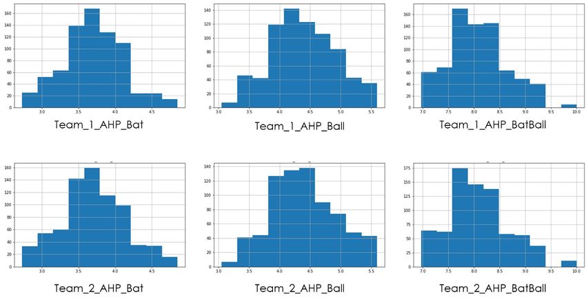
Tripathi et al. / Indian Journal of Science and Technology 2020;13(38):4013–4035

1 Introduction
The IPL (Indian Premier League) is a 20-20 cricket league in India where eight teams (representing eight cities in India) play
against each other. This game is India’s biggest cricket festival - the most celebrated and the most viewed, where the action is
just not limited to the cricket field. The clatters, promotional events, cheerleaders, advertisements, fan clubs, interactions, and
betting are celebrated along with the players and the matches.
    The entire revenue cycle of the IPL revolves around advertising. IPL also utilizes television timeouts, and there are other
humongous opportunities associated with advertising. Apart from national and global broadcasts, the matches are transmitted
to regional channels in eight different languages. The brand value of the IPL was |475 billion (US$6.7 billion) in 2019 (1) . The
IPL cricket league has proved to be a ’game-changer’ for both cricket and the entire Indian advertising industry (2) .
    ”Due to the saturated market, it is especially important for sports organizations to function with maximum efficiency and
to make smart business decisions” (3) . One of the most common areas where Sports organizations use analytic is assessing an
athlete’s value to their brand and strategizing their marketing activities.
    In this paper, models using machine learning to predict IPL matches’ outcomes were developed. Figure 1 illustrates the entire
process followed while conducting the research.
    During the research, a multi-step approach was taken to gather and pre-process the historical data. Feature engineering (4,5)
techniques were applied to derive more insights about the current dataset. Further, analysis of the essential features was done
using selection techniques, and simultaneously best players were marked based on their performances. Optimized features from
players’ performance were then added to the team data. The issue of multicollinearity, which occurs when multiple features are
highly linearly related was tackled. One of the main issues identified during the research was the symmetry in the dataset.
The models returning different results for the same input fed in two configurations was observed. This concept in the paper
is termed as model ambiguity, which occurs due to the model’s inability to interpret data symmetry because of its asymmetric
nature. The models were trained using multiple machine learning classification algorithms to develop a predictive model. The
highest accuracy was observed with Random Forest, i.e., 60.043%, with a standard deviation of 6.3% and 1.4% ambiguity.

Fig 1. Complete process from data scrapping to creating optimised model accuracies with reduced ambiguity for predicting IPL matches’
winner.

2 Related works
Many researchers have contributed towards predicting the results of cricket matches. Authors (6) proposed a paper on predicting
the outcome of an IPL match, where they acquired the dataset available for all the 11 seasons from the archives of the IPL
website (7) and applied the concept of Multivariate Linear Regression to calculate the strengths of a team using the data from
the Player Points section of the official IPL website. Later for prediction, the scholars utilized various classifiers, namely Naive
Bayes, Extreme Gradient Boosting, Support Vector Machine, Logistic Regression, Random Forests, and Multilayer perceptron.
In another study, authors (8) adopted the Team Composition method to predict the outcome of an ODI match. They utilized the

https://www.indjst.org/                                                                                                        4014
Tripathi et al. / Indian Journal of Science and Technology 2020;13(38):4013–4035

players’ data career statistics (both recent and overall performance) to calculate the player’s strength and aggregate to finalize
the team strength. They also included other features like venue and toss. The model derived from their research gives the best
result with the KNN algorithm.
    Although not related to cricket match prediction, the authors conducted a study (9) to predict the performance of bowlers.
They used Multilayer Perceptron and created a new feature using the data called CBR (Combined Bowling Rate) and calculating
the harmonic mean of the Bowling Average, Bowling Economy, and Bowling Strike Rate. Authors (10) used the pressure Index
of the team batting in the second innings to predict the match at different points of the chase; they devised a formula to calculate
the pressure index at each point and used various methods to calculate the probability of a win based on the pressure index.

3 Material and Methods
3.1 Dataset
3.1.1 Dataset gathering
The historical dataset was obtained from various sources – Kaggle (11) , ESPN Cricinfo (12) ,and iplt20 (7) . The performance data
of individual players was scraped from the ESPN Cricinfo website by using Python Library Beautiful Soup (13) to calculate each
player’s strength and the team. This scrapped data demonstrates 26 features - including batting and bowling performances of
the players. Additionally, match results data was obtained from Kaggle. This data displayed 18 features. The IPL winning point
table yearly data was accumulated from the IPL website. This data demonstrated the point feature.

3.1.2 Pre-processing of data
3.1.2.1 Conversion of data format (Label Encoding).
Most of the Machine Learning algorithms work better with numerical values than the string values. Hence, all the string formats
in the dataset were converted to the numerical formats utilizing the Label Encoding. The features that were converted: Team
Names, Venue Names, Winning Team Name, Toss Winner Team Name.

3.1.2.2 Data cleaning and dealing with null values.
To produce accurate results, all the unnecessary features from the dataset were eliminated, for example – Umpire Name, Stadium
Name, Date, Dl applied, Player of the match. The features that could result in data leakage, such as Win by Runs and Win by
Wickets, were excluded. Further, all the match rows that were dismissed, drawn, or null were eradicated.

3.1.3 Class imbalance

                  Fig 2. Historical data of the number of times each participating team has won a match during the IPL

   Class Imbalance is a problem in machine learning where the class distribution is highly imbalanced (14,15) . Predicting the
results using the team’s name was not feasible as it can cause a massive Class Imbalance between the groups. For example –
MI (Mumbai Indians) winning more than 100 matches whereas KTK (Kochi Tuskers Kerala) wining less than 10 matches is

https://www.indjst.org/                                                                                                       4015
Tripathi et al. / Indian Journal of Science and Technology 2020;13(38):4013–4035

a Class Imbalance problem. Refer to Figure 2. Hence, to rule out the class imbalance, the model was designed to predict the
winner based on the essential features instead of the Team names, declaring either Team 1 or Team 2 as a winner. Moreover, the
number of times Team 1 won is more than Team 2 was noticed. Further, to resolve this issue and balance the Team 1 winning
and Team 2 winning in the label column, few values of column Team 1 were interchanged with column Team 2.

3.1.4 Assumptions
A few assumptions to make the model accurate and robust were followed. The owners changed the names of few teams due
to legal actions or due to the change in the ownership; however, the players and team dynamics did not change. The name
Delhi Capitals was changed to Delhi Daredevils, Deccan Chargers to Sunrisers Hyderabad, and Pune Warriors to Rising Pune
Supergiant. In these cases, the same team irrespective of the change in the name was taken. Moreover, the data of only 11 players
for a team based on the highest number of matches they have played during the IPL was considered.
   Refer Table 1 for the features extracted from the gathered and pre-processed data.

                                          Table 1. Final features extracted from gathered data
 Player                   Mat                        Inns                     NO                 Runs
 HS                       Ave                        BF                       SR                 100
 50                       4’s                        6’s                      Overs              Mdns
 Wkts                     Econ                       Ct                       St
                                               a. Features extracted from ESPN Cricinfo
 Team                     Won                        Lost
 Tied                     Pts
                                                  b. Features extracted from IPL T20
 Season                   City                      Team_1                  Team_2
 Toss_Winner              Toss_Decision             Winner
                                                  c. Features extracted from IPL T20

3.2 Feature engineering
3.2.1 Base features
3.2.1.1 Features from the processed data:.
From the gathered and processed data, following three meaningful features were extracted.
   1. City 2. Toss Winner 3. Toss Decision
   Since the algorithms do not interpret string values, label encoding on the above three features was done, as follows:
   1. City: If the match is played on the home ground of Team 1, the city value is taken as zero. If the match is played on the
home ground of Team 2, then the city’s value is taken as 1, and if the match is played in some other city, then the city value is
taken as 2.
   2. Toss Winner: If the Toss is won by Team 1, the Toss Winner value is taken as zero. If the Toss is won by Team 2, the Toss
Winner value is taken as 1.
   3. Toss Decision: If the Toss winner chooses to Bat, the value of the Toss Decision is taken as zero, and if the Toss winner
chooses to Bowl, then the value of the Toss Decision is taken as 1.
For Base Feature Distribution, refer to Figure 3 .

                                               Fig 3. Feature distribution of base features

https://www.indjst.org/                                                                                                    4016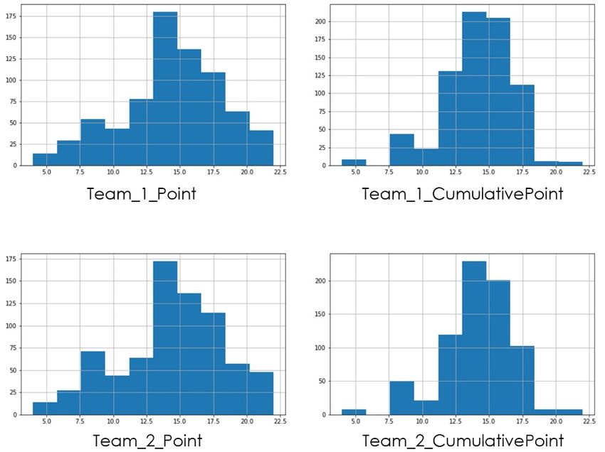
Tripathi et al. / Indian Journal of Science and Technology 2020;13(38):4013–4035

3.2.1.2 Dream 11 strength calculation.
In the first approach, the Dream11 points table was referred to derive the formula. For the definitions of point system and their
notations, refer to Appendix A (a, b, c, d).
3.2.1.2.1 Batting Score of a player
. Input: Players p ∈ P, Career Statistics of player p: φ (p)
   Output: Batsmen Score of all the players: φ Batsman Score

   1.   for all players p ∈ P do
   2.   φ ← φ (p)
   3.   u ← (1* ΦRuns_Scored) +(1*Φnum_4s) + (2*Φnum_6s) + (8*Φfifties) + (16*Φhundreds) - (2*Φfduck)
   4.   if Φbat_strike_rate < =50:
        v ← -6
        else if Φbat_strike_rate > 50 and Φbat_strike_rate < =60:
        v ← -4
        else if Φbat_strike_rate > 60 and Φbat_strike_rate < = 70:
        v ← -2
        endif
   5.   w ← v * Φbat_strike_rate* Φbat_innings
   6.   y←u+w
   7.   φ Batsman Score ← y
   8.   end for

3.2.1.2.2 Bowling Score of a player
. Input: Players p ∈ P, Career Statistics of player p: φ (p)
   Output: Bowling Score of all the players: φ Bowling_Score

   1.   for all players p ∈ P do
   2.   φ ← φ (p)
   3.   u ← (25*Φwickets) + ( 8*Φctchs) + (12*Φstmp) + (8*Φ4_wicket_haul ) + (16*Φ5_wicket_haul) + (8*Φmaidens)
   4.   if Φbowl_economy < = 6 and Φbowl_economy > 5:
        v←2
        else if Φbowl_economy > 4 and Φbowl_economy < = 5:
        v←4
        else if Φbowl_economy < = 4:
        v←6
        else if Φbowl_economy > = 9 and Φbowl_economy < 10:
        v ← -2
        else if Φbowl_economy >= 10 and Φbowl_economy < 11 :
        v ← -4
        else if Φbowl_economy >= 11:
        v ← -6
        endif
   5.   w ← v * Φbowl_economy* Φbowl_innings
   6.   y←u+w
   7.   φ Bowling_Score ← y
   8.   end for

3.2.1.2.3 Total Score of a player
. Input: Players p ∈ P, φ Bowling_Score, φ Batsman_Score
   Output: Total Strength← φ Total _Strength, φ Batsman_Strength, φ Bowling_Strength

   1. for all players p ∈ P, φ Bowling_Score, φ Batting_Score do

https://www.indjst.org/                                                                                                    4017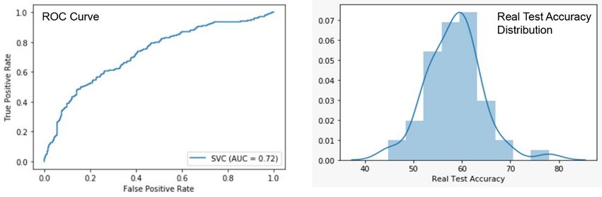
Tripathi et al. / Indian Journal of Science and Technology 2020;13(38):4013–4035

   2.   φ Total_Strength ← (φ Bowling_Score + φ Batting_Score) / φ tot_matches
   3.   φ Batsman_Strength ← φ Batting_Score / φ Bat_innings
   4.   φ Bowling_Strength ←φ Bowling_Score/ φ Bowl_innings
   5.   endfor

3.2.1.2.4 Team Strength
. Input: Top 11 Players p ∈ P, φ Total _Strength, φ Batsman_Strength, φ Bowling_Strength
   Output: Team Strength: φ Team _Strength

   1.   for all players p ∈ P , φ Total_Strength do
   2.   φ Team _Strength ← (∑ φ Total _Strength / φ max_matches)
   3.   φ Team_Batting_Strength ← (∑ φ Batsman _Strength / φ max_matches)
   4.   φ Team _Bowling_Strength ← (∑ φ Bowling _Strength / φ max_matches)
   5.   endfor

3.2.1.2.5 Cumulative Team Strength
. For a particular year, Team Strength represents the previous year’s performance, whereas the Cumulative Team Strength
signifies the mean of the Team Strength of all the last years. For example – for the Mumbai Indians in 2016, the Strength will
be the 2015 strength, and Cumulative Strength will be the mean of the Strength from 2008 to 2015. From this section, eight
significant features were collected, mentioned below:

 1. Team_1_BattingStrength                                          2. Team_2_BattingStrength
 3. Team_1_BowlingStrength                                          4. Team_2_BowlingStrength
 5. Team_1_Strength                                                 6. Team_2_Strength
 7. Team_1_CumulativeStrength                                       8. Team_2_CumulativeStrength

   For Dream 11 strength feature distribution, refer to Figure 4.

https://www.indjst.org/                                                                                                 4018
Tripathi et al. / Indian Journal of Science and Technology 2020;13(38):4013–4035

                                      Fig 4. Feature distribution of Dream 11 strength features

3.2.1.3 Analytic hierarchy process for strength calculation
. Different measures highlight different aspects of a player’s ability, which makes some features essential compared to others. For
example, the strike rate is a necessary feature for a game - especially T20. In T20, the number of overs is less, which makes this
feature more crucial as it adds to the team’s ability to score maximum runs. The features were weighted according to their relative
importance over other measures (features) in the research. The Analytic Hierarchy Process (AHP) was adopted to determine
these weights for each player to calculate their bowling and batting features. Besides, we calculated the weights for each team
based on their past performance.
   The Analytic Hierarchy Process is a method for decision-making in complex conditions in which many variables or criteria
are considered in prioritizing and selecting options (16) . AHP generates a weight for each evaluation criterion. The higher the
weight for a corresponding criterion, the more important is the corresponding criterion (Refer to Appendix B). Finally, the
AHP combines the criteria weights and the options amounts, thus determining a global score for each option and a consequent
ranking. The global score for a given option is a weighted sum of the scores it obtained with respect to all the criteria (17) .
3.2.1.3.1 Batting AHP
. Priority Order: The attributes were arranged in their decreasing order of importance based on the knowledge and experience
from the T20 cricket matches, as below:
   Batting Average > Innings > Strike Rate > 50’s > 100’s > 0’s
   Subsequently, a matrix was created to compare the importance of each attribute. Refer to Table 2.

                                                 Table 2. Criteria weights for Batting
 Batting         Average              INN                 SR                  50’s                100’s        0’s
 Average         1                    2                   3                   5                   6            7
 INN             0.5                  1                   2                   4                   5            6
 SR              0.333333             0.5                 1                   3                   4            5
 50’s            0.2                  0.25                0.333333            1                   2            3
 100’s           0.166667             0.2                 0.25                0.5                 1            2
 0’s             0.142857             0.166667            0.2                 0.333333            0.5          1

   Finally, from each attributed, weights were noted: Batting Average: 0. 3887, Innings: 0. 2601, Strike Rate: 0. 1754, Fifties: 0.
0834, Centuries: 0. 0550, Zeros: 0. 0373. Using these values the Batting strength through AHP was calculated.

AHP bat = 0.3887 ∗ Average + 0.2600 ∗ Innings + 0.1754 ∗ Strike Rate + 0.0834 ∗ 50′ s + 0.0550 ∗ 100′ s − 0.0373 ∗ 0′ s

3.2.1.3.2 Bowling AHP
. Priority Order: The attributes were arranged in their decreasing order of importance based on the knowledge and experience
from the T20 cricket matches, as below:
   Overs > Economy > Wickets > Bowling Average > Bowling Strike Rate > 4W Haul
   Subsequently, a matrix was created to compare the importance of each attribute. Refer to Table 3.
   Finally, the weights for each attributes were noted: Overs: 0.4174, Economy: 0.2634, Wickets: 0.1602, Bowling Average:
0.0975, Bowling Strike Rate: 0.067862, 4-Wickets Haul: 0.0615. Using these values the Bowling strength through AHP was

https://www.indjst.org/                                                                                                      4019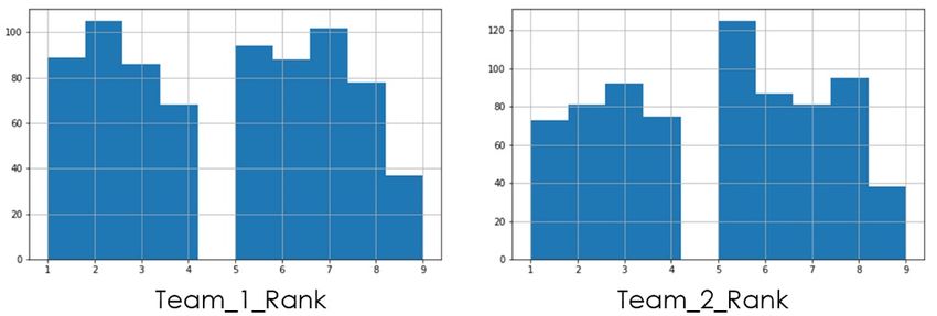
Tripathi et al. / Indian Journal of Science and Technology 2020;13(38):4013–4035
calculated.
AHP bowl = 0.387509 * Overs + 0.281308 * Economy + 0.158765 * Wickets + 0.073609 * Bowling Average + 0.067862 *
Bowling Strike Rate + 0.030947 * 4W Haul
Table 3. Criteria weights for Bowling
Bowling Overs Economy Wickets Bowling Avg Bowling strike rate 4W Haul
Overs 1 2 4 6 6 7
Economy 0.5 1 4 5 5 6
Wickets 0.25 0.25 1 4 4 6
Bowling Avg 0.166666 0.2 0.25 1 1 5
Bowling SR 0.166666 0.2 0.25 1 1 4
4W Haul 0.142857 0.166666 0.166666 0.2 0.25 1
From this section, four essential features were formed, mentioned below:
1. Team_1_AHP_Bat 2. Team_2_AHP_Bat
3. Team_1_AHP_Ball 4. Team_2_AHP_Ball
5. Team_1_AHP_BatBall 6. Team_2_AHP_BatBall
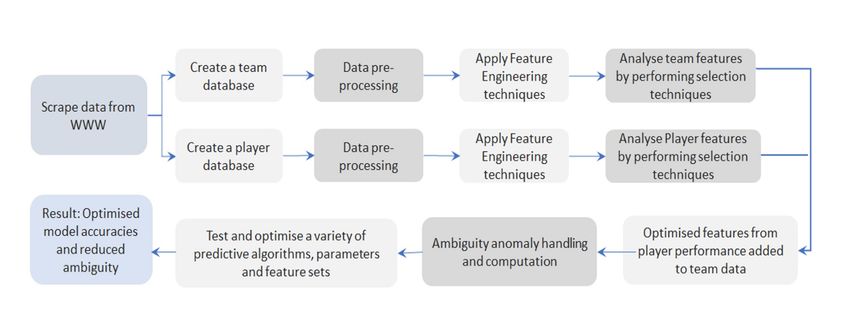
For AHP Strength Feature Distribution, refer to Figure 5 .
Fig 5. Feature distribution of AHP Strength features
3.2.1.4 Rank calculation using AHP
. Using the AHP, the coefficient for the win rate of each team against the other were derived. Assumption: KTK (Kochi Tuskers
Kerala) and GL(Gujrat Lions) Teams were dropped while calculating the weights, as they never played against each other.
Priority Order: The priority order through AHP with the dataset of the matches played for win/loss for each team against
each team was calculated. For example, the Team CSK (Chennai Super Kings) and MI (Mumbai Indians) played 27 matches
against each other, and according to the dataset, MI won 16, and CSK won the rest 11 games. In this instance, in the MI row,
the input will be 16/11 = 1.454545, and in the CSK row, it will be reciprocal, which is 11/16 or 1/1.4545454 = 0.6875. Refer to
Table 4.
https://www.indjst.org/ 4020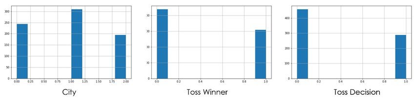
Tripathi et al. / Indian Journal of Science and Technology 2020;13(38):4013–4035

                                                  Table 4. Criteria weights for rank
 Rank       CSK             DD           KKR          KXIP           MI            RCB        RPS        RR           SRH
 CSK        1               2.5          1.857143     1.333333       0.6875        2.142857   2          2            2.142857
 DD         0.4             1            0.769231     0.642857       1             0.571429   1.25       0.72727      1
 KKR        0.538462        1.3          1            2.125          0.315789      1.4        3.5        1            1.888889
 KXIP       0.75            1.555556     0.470588     1              0.846154      1          1          0.9          0.846154
 MI         1.454545        1            3.166667     1.181818       1             1.777778   1.4        1            1.181818
 RCB        0.466667        1.75         0.714286     1              0.5625        1          3.5        0.7          0.785714
 RPS        0.5             0.8          0.285714     1              0.714286      0.285714   1          0.25         0.666667
 RR         0.5             1.375        1            1.111111       1             1.428571   4          1            1.5
 SRH        0.466667        1            0.529412     1.181818       0.846154      1.272727   1.5        0.66666      1

  Further, the yearly ranks of each team based on the win ratios was noted and the ranks were derived using AHP. Refer to
Table 5.
                                             Table 5. Ranks of teams derived from AHP
 Teams       RPS       DD       SRH        GL         KTK         RCB       KXIP     RR         KKR      MI        CSK
 Coefficients0.6043    0.8090   0.9042     1          1           1         0.9397   1.272      1.277    1.5188    1.6931
 Ranks       9         8        7          5          5           5         6        4          3        2         1

   For the KTK and GL, the mean value which is 1 as the coefficients was taken and two features were formed from this section,
as below:
   1. Team_1_Rank 2. Team_2_Rank
   For AHP Rank Feature Distribution, refer to Figure 6 .

                                          Fig 6. Feature distribution of AHP Rank features

3.2.1.5 Win rate
. For a cricket match, the win rate almost determines the overall performance of a team. A team is continuously winning the
matches against other teams is a sign that the team’s form is good and the probability of the team winning the upcoming matches
is higher. On the other hand, a losing team reflects that it is not in good form and may even lose games further.
    As next steps, the entire IPL match list played every year by each team from 2008 to 2019 was crawled. If the two teams
played against each other for the first time, the win rate was reset to 0 for both the teams. Subsequently, all the played matches
were checked and the winners for such occurrences were noted. This helped in defining a ratio for each team. For a match, the
past win rate ratio of the team was considered as below:

   Φwin_rate(Match R) = Total Number of wins till match R-1/ Total Number of matches played till R-1

   Two important features from this section were derived, as below:
   1. Team_1_Win_Rate 2. Team_2_Win_Rate
   For Win Rate Feature Distribution, refer to Figure 7.

https://www.indjst.org/                                                                                                     4021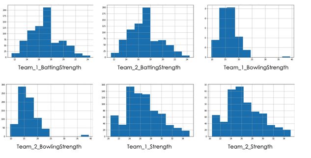
Tripathi et al. / Indian Journal of Science and Technology 2020;13(38):4013–4035
Fig 7. Feature Distribution of Win rate features
3.2.1.6 Team Points
. The IPL is a league tournament based on a point system. Every year, two teams play against each other twice before entering
the semi-final match, if not eliminated. The point table comprises teams, match won/lost/tied, and net run rate. Teams’ ranking
was done according to the teams’ points, and past performance features were fed to the model for predicting the results. Four
significant features were formed from this section as below:
1. Team_1_Point 2. Team_1_Cumulative Point
3. Team_2_Point 4. Team_2_Cumulative Point
For a particular year, Team Point represents the previous year’s performance, whereas the Cumulative Team Point represents
the mean of the strengths of all the previous years.
For Team Point Feature Distribution, refer to Figure 8.
Fig 8. Feature Distribution of Team Point features
3.2.2 Intersection Features
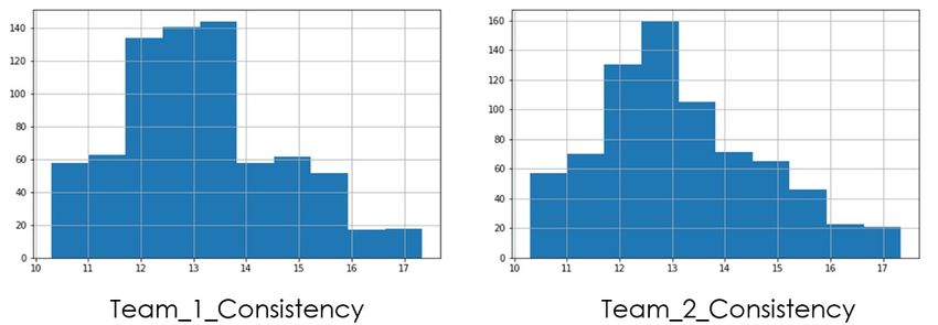
3.2.2.1 Consistency
. The consistency of a team adds more weightage to its current performance than the overall performance. Therefore, 80 percent
https://www.indjst.org/ 4022Tripathi et al. / Indian Journal of Science and Technology 2020;13(38):4013–4035
weightage was allotted to the current performance of a team and 20 percent weightage to their overall performance.
Team 1 Consistency = (Team 1 Strength ∗ 0.8 + Team 1 Cumulative Team Strength*0.2)/2
Team 2 Consistency = (Team 2 Strength ∗ 0.8 + Team 2 Cumulative Team Strength ∗ 0.2)/2
Two features were formed from this section, mentioned below:
1. Team_1_Consistency 2. Team_2_Consistency
For Consistency Feature Distribution, refer to Figure 9.
Fig 9. Feature Distribution of Consistency features
3.2.2.2 Win rate strength
. The individual strength of a team represents how strong a team is by considering the stats. However, various other factors
impact the winning of a team - for example - playing a team’s sequence, performance as a team, and sentiments of the audience.
This information was captured by multiplying the strength with the previous win rate of the team.
Team 1 Win Strength =Team 1 Win Rate ∗ Team 1 Strength
Team 2 Win Strength = Team 2 Win Rate ∗ Team 2 Strength
Team 1 Win Cumulative Strength = Team 1 Win Rate ” Team 1 Cumulative Strength
Team 2 Win Cumulative Strength = Team 2 Win Rate ” Team 2 Cumulative Strength
Four features were derived from this section, mentioned below:
1. Team_1_WinStrength 2. Team_1_WinStrength
3. Team_2_Win_Cumulative Strength 4. Team_2_Win_Cumulative Strength
For Win Strength Feature Distribution, refer to Figure 10.
https://www.indjst.org/ 4023Tripathi et al. / Indian Journal of Science and Technology 2020;13(38):4013–4035
Fig 10. Feature Distribution of Win Strength features
3.2.3 Transformation Features
With all the formulated Base and Intersection features, Transformed features were developed. These features were created by
subtracting two base features or intersection features from the same category. For example, Team1_Team_Strength is subtracted
from the Team2_Team_Strength to create a new feature.
Since many new features based was created on base and intersection features for the model, multicollinearity (18) could occur.
Multicollinearity occurs when multiple features in a model are highly linearly related, which means one variable can be predicted
quite accurately using the other variable. The problem with multicollinearity is that it causes the model to overfit. To deal with
multicollinearity in the derived model, all the base and intersection features that were used to create the new features were
dropped.
3.2.4 Addressing the Symmetry in Data
As per the primary assumption, every team’s performance is independent of the opposition team, toss decision, home-field
advantage, and progress into the series. This allowed to make independent team features that will be present in both TEAM1
and TEAM2. The features generated can be broadly bucketed into Match and Team Features. As there are similar features for
both TEAM1 and TEAM2, symmetry in the dataset was observed (Refer to Table 6 ).
Table 6. Example of a row from the dataset
Team1 Team 2 Team1_Strength Team2_Strength Winner Team1
CSK MI X Y 1 CSK
It is apparent to a human that while switching TEAM1 with TEAM2, the results will be the same. However, a machine
learning model is asymmetric in nature and is neither capable of identifying the symmetry of features nor has a way to input
the information about the symmetry of features. Hence, this information was entered to the model by generating a symmetric
duplicate for every row in the training set (Refer to Table 7 ).
Table 7. Mirroring the row from the dataset
Team1 Team2 Team1_Strength Team2_Strength Winner
CSK MI X Y 1
MI CSK Y X 0
The below steps were taken to the train and test sets:
1. The original dataset is split using train_test_split from sklearn (19) library into training and test sets. The data was split
such that 90% of data are in training set and 10% of data are in testing set.
2. The training set is then mirrored as shown above and append to the original training set which increases in training set
size
3. The test set is also mirrored but the test sets were not appended to create two test sets
https://www.indjst.org/ 4024Tripathi et al. / Indian Journal of Science and Technology 2020;13(38):4013–4035
3.2.5 Model Ambiguity
The mirroring of the rows only tells the model about the existence of a symmetric scenario, but the model will still interpret the
mirrored rows as new training set rows completely unrelated to the original rows. This asymmetric nature of the model leads
to ambiguity in the results in certain rows ( Refer to Table 8 ).
Table 8. Example of a match result and its mirrored data
Test Set Team1 Team2 Winner Prediction Team
1 KKR KXIP 1 1 KKR
2 KXIP KKR 0 1 KXIP
The model was tested for a given match in two configurations. The model interprets both the cases as two different test cases.
As a result, sometimes, the model returns different predictions for the same case. Such an occurrence is called Model Ambiguity.
Note: This occurrence is not an incorrect prediction, as the prediction will be counted correct in either test set 1 accuracy or
test set 2 accuracy.
To tackle this phenomenon of Model Ambiguity, the model was evaluated using five parameters apart from just training and
test accuracy:
• Training Accuracy: % of correct predictions in mirrored and merged train set
• Test 1 Accuracy: % of correct prediction in the original test set
• Test 2 Accuracy: % of correct prediction in the mirrored test set
• Real Test Accuracy: % of correct prediction after discrediting the scores for ambiguous rows
• Ambiguity: % of rows in which ambiguity is observed
The objective of hyperparameter tuning was to maximize real test accuracy by driving down the ambiguity while evaluating the
overfitting of the model using training accuracy and test 1 & 2 accuracies.
3.3 Data set split
Changing the random state in dataset the accuracy differs a lot was noted. This change occurs because the training and testing
dataset is randomly split based on the state in which the data was put. To prevent such a scenario and to make the model robust
RepeatedStratifiedKFold (20) was used. 10 folds and 2 iterations were selected to give a total of 20 folds. RepeatedStratifiedKFold
was preferred over StratifiedKFold (20) as dataset is small, and RepeatedStratifiedKFold gives more fold with larger validation
set.
Constant: Random State = 827 throughout the project was taken
The model was evaluated using accuracy and Standard Deviation, Cohen Kappa (21) , Skewness (22,23) and Kurtosis (22,23) . To
check or visualize the performance of the multi - class classification problem, AUC (Area Under The Curve) ROC (Receiver
Operating Characteristics) curves were plotted. These curves are one of the most important evaluation metrics for checking
any classification model’s performance (24).
4 Results and Discussions
8 Supervised algorithms to train the derived model were selected:
4.1 Model implementation using Naïve Bayes
The Real test accuracy of 58.233 % with a standard deviation of 5.5 % and ambiguity of 3.0% were derived (Refer to Table 9 ).
Table 9. Best results from Naïve Bayes
Ambiguity Real Test Accuracy Train Accuracy Cohen Kappa score
3.008 ± 2.5 % 58.233 ± 5.5 % 60.757 ± 0.9 % 0. 1891
The Area under the Curve is 0.63. The ROC curve was plotted with the best result using Naïve Bayes. The distribution of
Real Test Accuracy was done to derive Skewness and Kurtosis of the Real Test Accuracy (Refer to Figure 11 ).
• Kurtosis of the Real Test Accuracy is -0.7954
• Skewness of the Real Test Accuracy: -0.2357
https://www.indjst.org/ 4025Tripathi et al. / Indian Journal of Science and Technology 2020;13(38):4013–4035
Fig 11. ROC curve and real test accuracy distribution with Naïve Bayes
4.2 Model implementation using logistic regression
The model was tuned with over 1232 combinations. Refer to Appendix C (a). The best results derived: Real Test Accuracy of
57.78% with a standard deviation of 5.8% and ambiguity of 2.2 % (Refer Table 10 ).
Table 10. Best result with hyperparameters using logistic regression
penalty l2
solver liblinear
max_iter 400
tol 1
C 2
Ambiguity 2.199455± 1.4 %
Real Test Accuracy 57.77618± 5.8 %
Train Accuracy 61.11655± 3.2 %
Cohen Kappa score 0.1351
Further, the ROC curve with the best result was made and AUC value of 0.57 was derived. The Real test accuracy distribution
was plotted for deriving the Kurtosis and Skewness. Refer Figure 12.
• Kurtosis of the Real Test Accuracy: 0.5892
• Skewness of the Real Test Accuracy: 1.4699
Fig 12. ROC Curve and Real test accuracy distribution with Logistic Regression
https://www.indjst.org/ 4026Tripathi et al. / Indian Journal of Science and Technology 2020;13(38):4013–4035
4.3 Model implementation using support vector machines
The model was tuned with over 25 combinations. Refer to Appendix C (b). Real test accuracy of 58.416% with a standard
deviation of 5.69% and ambiguity of 0.24% was derived (Refer to Table 11 ).
Table 11. Best result with hyperparameters using support vector machines
c 0.1
Gamma 0.001
Kernal rbf
Ambiguity 0.24 ± 0.3%
Real Test Accuracy 58.416% ± 5.69%
Train Accuracy 61.13 ± 4.2%
Cohen Kappa score 0.1921
The Area under the Curve is 0.72. The ROC curve was plotted with the best result from Support Vector Machines. The
distribution of Real Test Accuracy was done to derive Skewness and Kurtosis of the Real Test Accuracy (Refer to Figure 13 ).
• Kurtosis of the Real Test Accuracy is 1.6979
• Skewness of the Real Test Accuracy: 0.4171
Fig 13. ROC Curve and Real test accuracy distribution with SVM
4.4 Model implementation using k- Nearest neighbours
The model was tuned with over 300 combinations. Refer to Appendix C (c). Real test accuracy of 53.472% with a standard
deviation of 5.2% and ambiguity of 1.90% was derived (Refer to Table 12 ).
Table 12. Best result with hyperparameters using Knn
n_neighbors 15
weights uniform
metrics manhattan
Leaf-size 20
Ambiguity 1.900 ± 1.1%
Real Test Accuracy 53.472% ± 5.2%
Train Accuracy 62.043 ± 4.8 %
Cohen Kappa score 0.1634
The Area under the Curve is 0.81. The ROC curve was plotted with the best result using Knn. The distribution of Real Test
Accuracy was done to derive Skewness and Kurtosis of the Real Test Accuracy (Refer to Figure 14).
https://www.indjst.org/ 4027Tripathi et al. / Indian Journal of Science and Technology 2020;13(38):4013–4035
• Kurtosis of the Real Test Accuracy is 0.0502
• Skewness of the Real Test Accuracy: -0.3635
Fig 14. ROC curve and real test accuracy distribution with KNN
4.5 Model Implementation using ADABOOST
The model was tuned with over 56 combinations. Refer to Appendix C (d). The best result with the corresponding hyper-
parameters were derived - Real test accuracy is 60.035% with a standard deviation of 6.2% and ambiguity of 5.4% (Refer to
Table 13 ).
Table 13. Best result with hyper parameters using ADABOOST
learning_rate 0.01
n_estimators 150
Ambiguity 0.402 ± 0.9 %
Real Test Accuracy 60.035 ± 6.2 %
Train Accuracy 62.127 ± 0.9 %
Cohen Kappa score 0.194
Further the ROC curve with the best result was made and the AUC value of 0.62 was derived. The Real test accuracy
distribution with ADABOOST was plotted for deriving the Kurtosis and Skewness (Refer Figure 15 ).
• Kurtosis of the Real Test Accuracy: -0.6021
• Skewness of the Real Test Accuracy: -0.4677
Fig 15. ROC curve and real test accuracy distribution for AdaBoostClassifier
https://www.indjst.org/ 4028Tripathi et al. / Indian Journal of Science and Technology 2020;13(38):4013–4035
4.6 Model Implementation using XGBOOST
The model was tuned with over 3600 combinations. Refer to Appendix C (e). The best result with the corresponding hyper-
parameters were derived - Real test accuracy is 55.42 % with a standard deviation of 5.9% and ambiguity of 7% (Refer to Table 14
).
Table 14. Best result with hyperparameters using XGBOOST
learning_rate 0.05
max_depth 4
min_child_weight 1
gamma 0
colsample_bytree 0.3
n_estimators 100
Ambiguity 7.098 ± 2.9 %
Real Test Accuracy 55.42 ± 5.9 %
Train Accuracy 78.079 ± 0.9 %
Cohen Kappa 0.228
Further the ROC curve with the best result was made and the AUC value of 0.62 was derived. The Real test accuracy
distribution with XGBOOST was plotted for deriving the Kurtosis and Skewness (Refer Figure 16 ).
• Kurtosis of the Real Test Accuracy is -0.8633
• Skewness of the Real Test Accuracies: 0.0456
Fig 16. ROC Curve and Real test accuracy distribution for XGBOOST
4.7 Model implementation using ExtraTreesClassifiers
The model was tuned with over 320 combinations. Refer to Appendix C (f). The best results derived: Real Test Accuracy of
59.506 % with a standard deviation of 5.9% and ambiguity of 4.3% (Refer to Table 15 ).
Table 15. Best result with hyperparameters Extra TreesClassifier
n_estimators 2100
max_depth 12
max_features log2
min_sample_leaf 12
Ambiguity 4.286 ± 2.0 %
Real Test Accuracy 59.506 ± 5.9 %
Train Accuracy 74.71 ± 0.5 %
Cohen Kappa 0.1864
https://www.indjst.org/ 4029Tripathi et al. / Indian Journal of Science and Technology 2020;13(38):4013–4035
Further the ROC curve with the best result was made and the AUC value of 0.64 was derived. The Real test accuracy
distribution with ExtraTreesClassifiers was plotted for deriving the Kurtosis and Skewness (Refer to Figure 17 ).
• Kurtosis of the Real Test Accuracy is -0.2121
• Skewness of the Real Test Accuracies: 0.5902
Fig 17. ROC Curve and Real test accuracy distribution for Extra TreesClassifier
4.8 Model Implementation using Random Forest Classifier
The model was tuned with over 1200 combinations (25) . Refer to Appendix C (g). The best result with the corresponding
hyper-parameters were derived - Real test accuracy is 60.043 % with a standard deviation of 6.3% and ambiguity of 1.4% (Refer
to Table 16 ).
Table 16. Best result with hyperparameters using Random Forest Classifier
max_features 0.5
bootstrap True
max_depth 3
min_samples_leaf 4
min_samples_split 2
colsample_bytree 0.3
n_estimators 1200
Ambiguity 1.404 ± 1.4 %
Real Test Accuracy 60.043 ± 6.3 %
Train Accuracy 65.978 ± 0.7 %
Cohen Kappa 0.1785
Further, the ROC curve with the best result was made and the AUC value of 0.62 was derived. The Real test accuracy distribution
with Random Forest Classifier was plotted for deriving the Kurtosis and Skewness (Refer to Figure 18 ).
• Kurtosis of the Real Test Accuracy is -0.8606
• Skewness of the Real Test Accuracies: -0.2491
https://www.indjst.org/ 4030Tripathi et al. / Indian Journal of Science and Technology 2020;13(38):4013–4035
Fig 18. ROC Curve and real test accuracy distribution for Random Forest Classifier
5 Conclusion and Future Works
The research focused on predicting the winner for an IPL match using machine learning and utilizing the available historical
data of IPL from season 2008-2019. In the process, various Data Science methods were adopted to conduct the study, including
data mining, visualization, preparation of database, feature engineering, applying the Analytic hierarchical process, creating
prediction models, and training classification techniques.
The IPL dataset was gathered and pre-processed. The missing values were removed, and variables were encoded into the
numerical format to make the dataset uniform. The essential features were then derived from data using the domain knowledge
to extract raw data features via data mining techniques, and the results were derived from the model. Since the dataset that is
available for IPL is limited and small, multiple levels of features were created to make sure that the derived model is not underfit.
Almost every feature that can affect the result of a match was derived. Further, the problem of multicollinearity was solved and
the issue of data symmetry was identified (termed as model ambiguity). Several machine learning models were applied to the
selected features to predict the IPL match results. The best results were concluded using the tree-based classifiers. The highest
accuracy of 60.043% with Random Forest with a standard deviation of 6.3% and an ambiguity of 1.4% was observed (Refer to
Table 17 ).
Table 17. Accuracies from various algorithms with their ambiguity and Cohen KappaScore
Algorithm Accuracy Cohen Kappa Ambiguity
Naïve Bayes 58.23 ± 5.5 % 0.19 3.00 %
Adaboost 60.03 ± 6.2 % 0.19 0.40%
Logistic Regression 57.77± 5.8 % 0.13 2.20%
Support Vector Machines 58.42% ± 5.69% 0.19 0.24%
Knn 53.47% ± 5.2% 0.16 1.90%
XGBoost 55.42 ± 5.9 % 0.23 7.10 %
Extra Trees Classifier 59.51 ± 5.9 % 0.19 4.30%
Random Forest Classifier 60.04 ± 6.3 % 0.18 1.40%
In this research, the player’s series-wise performance rather than their match-wise performance was taken while calculating
the player’s strength. For a more thorough approach to further develop this research, match wise data can be considered. The
research can also be further enhanced by adding other factors like comparing players’ performances at a particular stadium.
Appendices
Appendix A: Dream 11 Point Tables
a. Score Point Table:
https://www.indjst.org/ 4031Tripathi et al. / Indian Journal of Science and Technology 2020;13(38):4013–4035
Notation Type of Points Weight
φ Matches Being a part of the starting XI 4
φ Runs_Scored Every run scored 1
Φctchs Total catches taken 8
Φfifties Total number of 50s scored 8
Φhundreds Total number of 100s scored 16
Φnum_4s Total number of 4s scored 1
Φnum_6s Total number of 6s scored 2
φ stmp Stumping/ Run Out (direct) 12
Φr_out Run Out (Thrower/Catcher) 8/4
Φfduck Dismissal for a Duck (only for batsmen, wicket-keepers and all-rounders) -2
Φbat_innings Number of times a player has batted in a match
Φbowl_innings Number of times a player has bowled in a match
Φwickets Number of wickets taken by a bowler in the season 25
Φmaidens Number of times a bowler has bowled an over without conceding any runs 8
Φ4_wicket_houl Number of times a player has taken 4 wickets in a single match 8
Φ5_wicket_houl Number of times a player has taken 5 wickets in a single match 16
Φbowl_economy Bowling economy of a player
Φbat_strike_rate Batting Strike Rate of a player
Φmax_matches Maximum matches played by a team
b. Bonus Points
Type of Points Weight
Every boundary hit 1
Every six-hit 2
Half-Century (50 runs scored by a batsman in a single inning) 8
Century (100 runs scored by a batsman in a single inning) 16
Maiden Over 8
4 wickets 8
5 wickets 16
c. Economy Rate
Type of Points Weight
Minimum overs bowled by a player to be applicable 2 overs
Between 6 and 5 runs per over 2
Between 4.99 and 4 runs per over 4
Below 4 runs per over 6
Between 9 and 10 runs per over -2
Between 10.01 and 11 runs per over -4
Above 11 runs per over -6
d. Strike Rate
Type of Points Weight
Minimum balls faced by a player to be applicable 10 balls
Between 60 and 70 runs per 100 balls -2
Continued on next page
https://www.indjst.org/ 4032Tripathi et al. / Indian Journal of Science and Technology 2020;13(38):4013–4035 Table 19 continued Between 50 and 59.99 runs per 100 balls -4 Below 50 runs per 100 balls -6 Appendix B: Analytical Hierarchy Process Scale Table Appendix C: Hyperparameters used for training our model a. Hyperparameters for Logistic Regression penalty l2, l1 solver liblinear max_iter 100, 200, 300, 400, 600, 900, 1200, 1500, 1800, 2100 tol 0.0001, 0.00001, 0.0005, 0.001, 0.1, 0.5, 1 C 1.0, 1.5, 2, 1.25, 1.75, 3, 4, 5, 7, 9 ,12 b. Hyperparameters for Support Vector Machines Kernel rbf Gamma 1, 0.1, 0.01, 0.001, 0.0001 C 0.1, 1, 10, 100, 1000 Hyperparameters for Knn n-neighbors 1, 3, 5,6, 8, 10,12, 14, 15, 18 Weights uniform, distance Metric euclidean, manhattan, hamming Leaf_Size 10, 15,20, 25,30 c. Hyperparameters for Adaboost learning_rate 0. 005 ,0.01 ,0.02, 0.05,0.15, 0.5, 0.1,1 n_estimators 10,20,50,100,200,800,1000 https://www.indjst.org/ 4033
Tripathi et al. / Indian Journal of Science and Technology 2020;13(38):4013–4035

d. Hyperparameters for XGboost

 learning_rate                                                        0.05, 0.10,0.15, 0.25
 n_estimators                                                         50,100,200,500,700,1000
 max_depth                                                            4,5,6,7,8
 gamma                                                                0,0.1, 0.2,0.3
 min_child_weight                                                     1,3
 colsample_bytree                                                     0.3, 0.4, 0.7

   e. Hyperparameters for ExtraTreeClassifier

 n_estimators                                            100,200,600,900,1200,1500,1800,2100
 max_depth                                               3,4,5,12,15
 max_features                                            Sqrt, log2
 min_sample_leaf                                         3,5,8,12

   f. Hyperparameters for RandomForestClassifier

 bootstrap                                                                 True, False
 max_depth                                                                 3,4,5,6,7
 max_features                                                              0.5, ’sqrt’,’log2’
 min_samples_leaf                                                          2, 4
 min_samples_split                                                         2, 5
 criterion                                                                 Gini, entropy
 n_estimators                                                              800,1000,1200,1600,2000

References
 1) Gupta V, Santosh N. Duff & Phelps Launches IPL Brand Valuation Report. 2019. Available from: https://www.duffandphelps.com/about-us/news/ipl-
    brand-valuation-report-2019.
 2) Badwe A. IPL Advertising: All you need to know about the game of revenue. Kreedon. 2019. Available from: https://www.kreedon.com/ipl-advertising-
    all-you-need-to-know/.
 3) Fried G, Mumcu C. Sport analytics: A data-driven approach to sport business and management. and others, editor;Taylor & Francis. 2016. Available
    from: https://doi.org/10.4324/9781315619088.
 4) Heaton J. An empirical analysis of feature engineering for predictive modeling. In: SoutheastCon, Norfolk, VA. 2016;p. 1–6. Available from:
    https://doi.org/10.1109/SECON.2016.7506650.
 5) Zheng A, Casari A. Feature engineering for machine learning: principles and techniques for data scientists. O’Reilly Media. 2018.
 6) Lamsal R, Choudhary A. Predicting Outcome of Indian Premier League (IPL) Matches Using Machine Learning. 2018. Available from: https:
    //arxiv.org/abs/1809.09813.
 7) IPL website. . Available from: https://www.iplt20.com.
 8) Jhanwar MG, Pudi V. Predicting the Outcome of ODI Cricket Matches: A Team Composition Based Approach. In: and others, editor. European Conference
    on Machine Learning and Principles and Practice of Knowledge Discovery in Databases. 2016. Available from: https://api.semanticscholar.org/CorpusID:
    35555185.
 9) Saikia H, Bhattacharjee D, Lemmer HH. Predicting the Performance of Bowlers in IPL: An Application of Artificial Neural Network. International Journal
    of Performance Analysis in Sport. 2012;12(1):75–89. Available from: https://dx.doi.org/10.1080/24748668.2012.11868584.
10) Bhattacharjee D, Talukdar P. Predicting outcome of matches using pressure index: evidence from Twenty20 cricket, Communications in Statistics -
    Simulation and Computation. 2019. Available from: https://doi.org/10.1080/03610918.2018.1532003.
11) Kaggle. . Available from: https://www.kaggle.com/manasgarg/ipl.
12) ESPNCricInfo. . Available from: https://stats.espncricinfo.com/.
13) Beautiful Soup Python Library. . Available from: https://pypi.org/project/beautifulsoup4/.
14) Brownlee J. A Gentle Introduction to Imbalanced Classification. Machine Learning Mastery. 2019. Available from: https://machinelearningmastery.com/
    what-is-imbalanced-classification/.
15) Johnson JM, Khoshgoftaar TM. Survey on deep learning with class imbalance. Journal of Big Data. 2019;6(1). Available from: https://dx.doi.org/10.1186/
    s40537-019-0192-5.

https://www.indjst.org/                                                                                                                            4034
Tripathi et al. / Indian Journal of Science and Technology 2020;13(38):4013–4035
16) Emrouznejad A, Ho W. Fuzzy Analytic Hierarchy Process. and others, editor;NewYork. Chapman and Hall/CRC. . Available from: https://doi.org/10.
1201/9781315369884.
17) Passi K, Pandey N. Increased prediction accuracy in the game of cricket using machine learning. International Journal of Data Mining & Knowledge
Management Process(IJDKP). 2009;8(2). Available from: https://arxiv.org/abs/1804.04226.
18) Gokmen S, Dagalp R, Kilickaplan S. Multicollinearity in measurement error models. Communications in Statistics - Theory and Methods. 2020;p. 1–12.
Available from: https://dx.doi.org/10.1080/03610926.2020.1750654.
19) SKLearn. . Available from: https://scikit-learn.org/.
20) Kohavi R. A study of cross-validation and bootstrap for accuracy estimation and model selection. In: International Joint Conference on Artificial
Intelligence;vol. 14. 1995;p. 1137–1145. Available from: http://ai.stanford.edu/~ronnyk/accEst.pdf.
21) Vieira SM, Kaymak U, Sousa MCJ. Cohen’s kappa coefficient as a performance measure for feature selection. International Conference on Fuzzy Systems.
2010. Available from: https://doi.org/10.1109/fuzzy.2010.5584447.
22) Blanca MJ, Arnau J, López-Montiel D, Bono R, Bendayan R. Skewness and Kurtosis in Real Data Samples. Methodology. 2013;9(2):78–84. Available from:
https://dx.doi.org/10.1027/1614-2241/a000057.
23) Cain MK, Zhang Z, Yuan KH. Univariate and multivariate skewness and kurtosis for measuring nonnormality: Prevalence, influence and estimation.
Behavior Research Methods. 2017;49(5):1716–1735. Available from: https://dx.doi.org/10.3758/s13428-016-0814-1.
24) Narkhede S. Understanding AUC - ROC Curve. Towards Data Science. 2018. Available from: https://www.48hours.ai/files/AUC.pdf.
25) Probst P, Wright MN, Boulesteix AL. Hyperparameters and tuning strategies for random forest. Wiley Interdisciplinary Reviews: Data Mining and
Knowledge Discovery. 2019;9(3). Available from: https://dx.doi.org/10.1002/widm.1301.
https://www.indjst.org/ 4035You can also read