THE IMPACT OF TRADE POLICY UNCERTAINTY SHOCKS ON THE EURO AREA - MUNICH PERSONAL REPEC ARCHIVE
←
→
Page content transcription
If your browser does not render page correctly, please read the page content below
Munich Personal RePEc Archive

The impact of trade policy uncertainty
shocks on the Euro Area

Arigoni, Filippo and Lenarčič, Črt

1 June 2020

Online at https://mpra.ub.uni-muenchen.de/100832/
MPRA Paper No. 100832, posted 05 Jun 2020 10:38 UTC
The impact of trade policy uncertainty
                      shocks on the Euro Area∗
                         Filippo Arigoni†                 Črt Lenarčič‡

                                            May 2020

                                             Abstract

       This paper sets up a Bayesian SVAR model on Euro Area data and identifies

       trade policy uncertainty shocks using a minimum set of sign restrictions. We

       find that rising trade policy uncertainty adversely affects the real business cycle

       in the Euro Area mostly in short term, while it has more persistent effects on

       the Euro effective exchange rate and, to a lesser extent, on prices. In line with

       the recent geo-political events, the evidence suggests an increasing contribution

       to Euro Area fluctuations towards the end of the sample period. The results

       are robust to alternative measures of trade policy uncertainty. Furthermore, we

       show that sectors exhibit heterogeneous responses to trade policy uncertainty

       shocks.

       Keywords: Trade policy uncertainty; Euro Area; uncertainty shocks; Bayesian
       SVAR; sign restrictions.

       JEL Classification: C32, D80, E30, F13.
   ∗
     The views presented herein are those of the authors and do not necessarily represent the official
views of Bank of Slovenia or of the Eurosystem.
   †
     Bank of Slovenia, Analysis and Research Department, author’s e-mail account: fil-
ippo.arigoni@bsi.si
   ‡
     Bank of Slovenia, Analysis and Research Department, author’s e-mail account: crt.lenarcic@bsi.si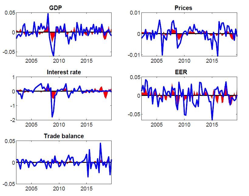
1    Introduction

Many developments in the global geo-political environment have prompted a renewed
discussion on the role of policy uncertainty on particular economies. We can regard
the Brexit vote, the height of the sovereign debt crisis in Europe, the economic policy
uncertainties, and after all the outbreak of the US-China trade war starting in 2018
as one of the main factors that have shaped economic activities over the last couple
of years. Indeed, these events had paved the way for the tightening of trade condi-
tions severely, which have curbed economic exchanges at global level. The first main
contribution related to quantifying the economic relevance of such an environment is
provided by Caldara et al. (2020). In their application on the US economy, they study
the effects of trade policy uncertainty (henceforth, TPU), highlighting the magnitude
of real impacts and stressing evidence of contraction for business investment.
In this paper, we analyze the reaction of the Euro Area (henceforth, EA) business
cycle to TPU shocks. To this aim, we estimate a number of structural shocks identi-
fied with a minimum set of sign restrictions in a Bayesian SVAR model setting. We
rely on Furlanetto et al. (2019) when deciding to use the sign restriction methodol-
ogy to identify uncertainty shocks. The choice to identify several shocks relies on two
important aspects. First, it allows to disentangle the source of fluctuations driving
the state of the economy in the region considered, over the sample period. Second
and more importantly, it reduces the issue that arises from sign restrictions, i.e. the
so-called ”multiple shocks problem” (Fry and Pagan, 2011; Furlanetto et al., 2019).
As in Furlanetto et al. (2019), sign restrictions are used to identify, among the other
shocks, uncertianty shocsl.
The exact purpose of the paper is to understand the effects that TPU may have on
economically relevant actors, like the EA. The employment of the EA as our study
case for this application is motivated by various reasons. First, as suggested by Figure
1, the EA openness (sum of exports and imports as percent of GDP) has substantially
increased over the last 15 years, reinforcing the dependence of the EA to global mar-

                                           1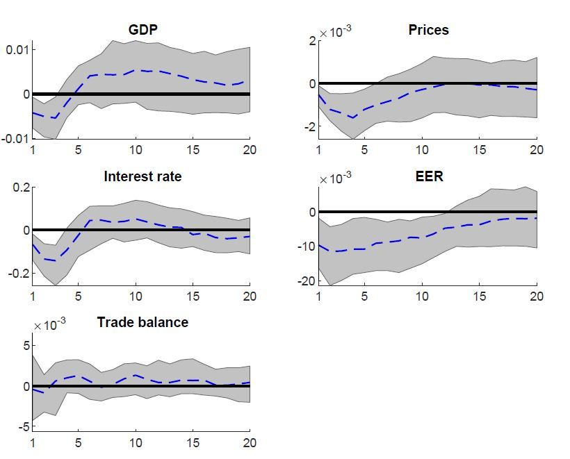
ket events. Second, the proportion of EA trade activities with the US and China has
also risen significantly over the last decade, strengthening the weight of the two trad-
ing partners for the domestic economy and boosting the possibility of cross-country
economic spillovers. Furthermore, the Brexit situation will soon represent another
non-negligible source of fluctuations for EA trade-related activities and it will gain
greater relevance in the very near future, especially at the point of policy decisions.

Figure 1: Openness of the EA, US and Chinese economies - sum of exports and imports
as percent of GDP (yearly data)

                                   Source: World Bank.

The measurement of trade policy uncertainty is performed by including the news-based
index of aggregate TPU developed by Caldara et al. (2020). To build the index, Cal-
dara et al. (2020) collected articles about topics related to TPU from the seven main
US newspapers and quantitatively aggregate them according to some factors which
are reported in detail in their paper. The TPU index is plotted in Figure 2 and it
covers the period between 1996:Q1 and 2019:Q3. It can easily be seen that along its
dynamics, periods of upswings of uncertainty in trade policies are present. This is

                                           2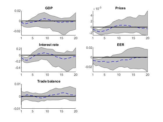
particularly evident in the recent years with the onset of the US-China trade war, as
the index has risen way above its historical median.1 The analysis of the Euro Area
is complemented with the identification of other shocks, either nominal or real, either
domestic or global.
The empirical results suggest the following main findings. First, we find that TPU
shocks have significant effects on the EA and especially on prices and mostly on the
Euro effective exchange rate (henceforth, Euro EER). Second, replacing the TPU in-
dex with a different measure of TPU confirms the robustness of our baseline evidence.
Moreover, we show that TPU shocks have a non-homogeneous magnitude on the real
activities, according to the sector that we consider.

                          Figure 2: Trade policy uncertainty index

                                   Source: Caldara et al. (2020)

With regard to the existing literature, several authors have already studied the eco-
nomic effects of different types of policy uncertainties. Put broadly, there are two
   1
     We depict the median of the TPU index since the latest (trade policy) developments significantly
affect the mean values of the index.

                                                 3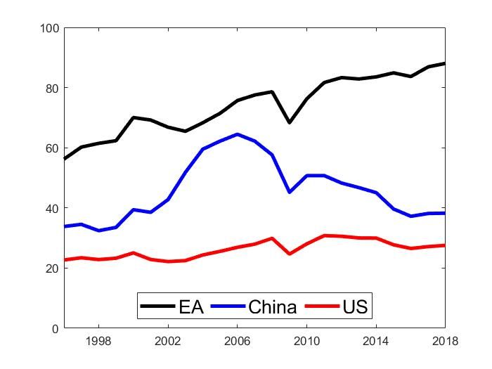
strands of literature. On the empirical side, the focus of the literature is mainly
related to the measurement of the policy uncertainties. Fernández-Villaverde et al.
(2015), for instance, study the effects of changes in uncertainty about future fiscal
policy (fiscal volatility shocks) on aggregate economic activity in the US. In order to
construct an indicator of fiscal volatility, they apply a law motion equation for fiscal
policy instruments that feed into a New Keynesian business cycle model calibrated to
the US economy. Baker et al. (2016), on the other hand, develop an index of economic
policy uncertainty (EPU index) that is based on newspaper coverage frequency. Sim-
ilarly, Rice (2020) constructs an Irish version of the EPU index. Hassan et al. (2019)
analyze the quarterly earnings conference-call transcripts to construct firm-level mea-
sures of the extent and type of political risk faced by firms listed in the US and how
it varies over time. Caldara et al. (2020) focus their research on constructing a trade
policy uncertainty indicator (TPU index) that uses newspaper coverage, firms’ earning
calls and tariff rates setting a study case for the US economy.
The theoretical strand of the literature focuses on the construction and use of several
types of theoretical models. Jaimovich and Rebelo (2009) propose a one-sector model
that is able to produce aggregate and sectoral co-movement in responses to contem-
poraneous and news shocks about fundamentals by introducing a capital utilization
variable, the investment adjustment costs and a weak wealth effect on the labour sup-
ply and at the same time overcoming the criticism of Barro and King (1984). Building
upon the theoretical work of Bloom (2009), Basu and Bundick (2017) and Fernández-
Villaverde et al. (2015) study the macroeconomic effects of uncertainty shocks in a
New Keynesian business cycle model setting. Colombo (2013) uses a SVAR model set-
ting in order to estimate the effects of a US economic policy uncertainty shock on EA
macroeconomic aggregates. Caggiano et al. (2017, 2020) estimate US economic policy
uncertainty shocks by using a nonlinear VAR approach. They confirm asymmetric
spillover effects, especially that the macroeconomic aggregates react more strongly to
uncertainty shocks in the periods of economic busts. They complement the results
shown in Caggiano et al. (2014) and Nodari (2014).

                                           4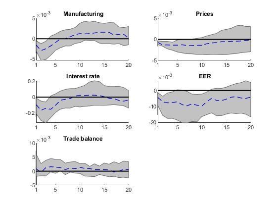
Based on the recent global trade developments, there is a growing literature explic-
itly studying the effects of trade policy uncertainty and news about the trade policy,
especially between the US and Chinese economies. Handley (2014) provides evidence
that the impact of trade policy uncertainty has on exporters based on a dynamic het-
erogeneous firms model. Handley and Limão (2017) and Crowley et al. (2018) papers
study the impact of trade policy on China’s export boom to the US following its 2001
World Trade Organisation (WTO) accession. Steinberg (2019), on the other hand,
estimates the effects of Brexit for the UK economy. Ebeke and Siminitz (2018) focus
their analysis on the effects of the trade policy uncertainty on investment in the EA.
They assume that economies that are more dependent on global trade networks show
a higher investment sensitivity with regards to the trade policy uncertainty.
The rest of the paper is organized as follows. Section 2 presents the theory and the
methodology of the Bayesian VAR model. Section 3 discusses the results of the esti-
mation of the baseline model and provides an alternative view of the model. Section
4 concludes.

2     Methodology

2.1    Model

This subsection provides the econometric methodology of a Bayesian SVAR model. In
general, Bayesian VAR models impose prior restrictions over the parameters’ distri-
bution of a VAR model. The model parameters are obtained by combining the prior
distribution with information obtained from the data. Bayesian VAR models became
increasingly popular since VAR models can usually suffer from a short data sample
problem, thus having low degrees of freedom space. In contrast to VAR models, the
Bayesian VAR model methodology enables us to include a larger number of explana-
tory variables in the time-series analysis. The possible limitation of the number of
time observations of separate variables in the model affects only the setting up the

                                          5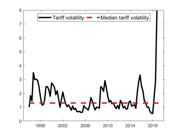
tightness of the priors used in the Bayesian VAR methodology. As mentioned before,
Bayesian methods were popularized in recent years reflecting the progress made in
the econometric and computational tools. The usage of prior information provides a
consistent way for forecasting exercises, despite that the choice of prior information
could be subjective.
We follow the Furlanetto et al. (2019) Bayesian SVAR model setting. The reduced
form VAR model is then given by

                                               P
                                               X
                                    yt = c +          Bi yt−i + ut                                (1)
                                               i=1

where the term yt represent a (N × 1) vector of N endogenous variables. The term
c is a (N × 1) vector of constants. The terms Bi are (N × N ) parameter matrices,
where i =, ..., P and P represents the number of lags in the model. The vector ut is
the (N × 1) reduced form residual where ut ∼ N (0, Σ). Σ is the variance-covariance
matrix. Bayesian methods are used for the estimation of the above model, while the
variables enter the model in levels. As in Furlanetto et al. (2019), we specify diffuse
priors so that the information in the likelihood is dominant. These priors lead to a
Normal-Wishart posterior with a mean and variance parameters corresponding to the
OLS estimates. Additional details are reported in the Appendix.2

2.2     Sign restrictions

An important part of the paper is the identification procedure. We can write the
prediction error, denoted as ut , as a linear combination of structural innovations ǫt

   2
    The Bayesian methodology is based on the likelihood function that follows a Gaussian distribution
regardless of the presence of non-stationarity. Therefore, it does not need to take special account of
non-stationarity (Sims, Stock, and Watson, 1990; Sims and Uhlig, 1991).

                                                  6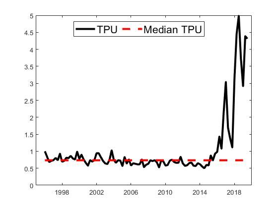
ut = Aǫt                                  (2)

where for ǫt ∼ N (0, I) holds and where the term I represents an (N × N ) identity ma-
trix. The term A is a non-singular parameter matrix, so that for variance-covariance
matrix the following structure applies, Σ = AA′ . As the variance covariance matrix
is symmetric, N (N − 1)/2 further restrictions are needed to derive A from this rela-
tionship (Furlanetto et al., 2019).
There are several ways to impose restrictions on the parameter matrix A. In the
identification procedure of the Cholesky decomposition, for instance, we restrict the
parameter matrix A to be lower triangular, which implies a recursive identification
scheme. In our case, the recursive identification scheme is not particularly theoreti-
cally convenient since the model estimation includes some of the fast-moving variables,
such are the overnight interbank interest rate (Eonia index) and the Euro EER.3 This
leads us to use an alternative identification procedure that is based on sign restrictions
(Faust, 1998; Canova and De Nicoló, 2002; Peersman, 2005; Uhlig, 2005; Fry and Pa-
gan, 2011) which is however used by Furlanetto et al. (2019) to identify financial and
uncertainty shocks.
The use of the identification procedure with sign restrictions is particularly helpful
when we deal with a larger number of shocks despite the fact that there are challenges
from a computational perspective. As already anticipated, the identification selection
of different shocks is based on two important aspects. First, it allows to obtain a clear
picture of the main occurrences impacting the EA. Second, it reduces the issue that
can arise from the sign restrictions approach, i.e. the so-called ”multiple shocks prob-
lem”, which arises when sign restriction methodology is applied (see Fry and Pagan,
2011 and Furlanetto et al., 2019). This relates to the fact that the sign restrictions
  3
      Similarly as in Rigobon and Sack (2003) and Bjørnland and Leitemo (2010).

                                                 7
imposed are potentially consistent with more than one shock. The ”multiple shocks
problem” is especially relevant when only one shock is identified. On the other hand,
it is arguably less serious in a model with several identified shocks (Furlanetto et al.,
2019).
Table 1 presents the restrictions used in the baseline model. It is worth saying that
restrictions are imposed only on impact (Canova and Paustian, 2011). Following Peers-
man (2005) and Peersman and Straub (2006), among others, we assign similar sign
restrictions to the demand, supply and monetary policy shocks (Table 1). To deal
with potential issues of endogeneity, we assume that demand, supply and monetary
policy shocks do not have a preferable sign restriction on the TPU index. In more
detail, a positive demand shock increases the output, prices and Euro EER. The in-
terest rates consequently respond with an increase as well. On the other hand, trade
balance is affected negatively as the positive demand shock increases the need for
economy’s imports while rising prices and Euro EER make domestic economy exports
less attractive abroad. We also do not assign a sign restriction for TPU index when a
demand shock hits the economy. A positive supply shock increases output, but, due
to product abundance, decreases prices. Consequently, the Euro EER and interest
rate have room to decrease. For the effect of the supply shock on the trade balance
we assume that there are no restrictions as import and export dynamics might cancel
each other out. As typically in the economic theory, a positive (restrictive) monetary
policy shock decreases output, trade balance and prices, while the interest rate and
Euro EER increase. Foreign shocks (commodity shocks and foreign demand shocks)
are also identified to cover additional and non-negligible dynamics which virtually im-
pact the EA business cycle.
Sign restrictions for the identification of the TPU shock have to be well thought out.
In contrast to most of the uncertainty literature, our paper focuses on a narrower
definition of uncertainty, i.e. the trade policy uncertainty, which is more specific to in-
ternational trade and economic activity. This allow us to take advantage of dissecting
the effects of trade policy uncertainties on economic activity of a particular economy
8in comparison to a reliance on a more general measure of uncertainty carrying various
dimensions that are difficult to interpret. In this perspective, we partly follow the
considerations made by Nodari (2014) and Baker et al. (2016) with respect to the
effects of the financial regulation policy uncertainty (FRPU) index on the macroeco-
nomic variables. An increase in the FRPU index decreases the industrial production
and prices. Fed responds by decreasing the key rate. On the other hand, the unem-
ployment rate and bond spreads increase. However, in order to disentangle the shocks
between demand and trade policy we consider additional variables in the model such
as trade balance and TPU index nevertheless. A positive TPU shock thus negatively
affects GDP and prices (see Table 1). Consequently, the monetary policy reacts with
a decrease in the key interest rates. The Euro EER decreases as well. On the contrast
to the case with the demand shock the trade balance variable in the case of a TPU
shock depends both on exports and imports, as they may cancel each other out if GDP
and Euro EER decrease (or increase) at the same time.
Table 1: Sign restrictions in the model
Trade Demand Supply Monetary Commodity Global
Variable uncert. policy demand
TPU + NA NA NA NA NA
GDP – + + – – +
Prices – + – – – NA
Interest rate – + – + – NA
Euro EER – + – + + +
Trade balance NA – NA – – +
*Note: The restrictions used for each variable (in rows) to the identified shocks (in columns).
2.3 Data
Before we move to the results of the model, lets shortly present the descriptive statis-
tics of the macroeconomic variables entering the model (Table 2). The number of
observations of the variables deviates between 92 and 95 due to different lengths of
the quarterly time series. The observations of all time series start from 1996:Q1, while
9the last observation for all the variables is 2019:Q3, except for the tariff volatility
index that is only available until 2018:Q4. The TPU and the tariff volatility indices
are taken from Caldara et al. (2020) paper. The EA GDP indicator is given as the
chain linked volumes index based on 2015 constant prices and is expressed in trillions
of Euro. Similarly to the EA GDP, the EA trade balance indicator variable is also
expressed in trillions of Euro. The nominal variables are the EA HICP index with a
base year of 2015, the Eonia index and the Euro EER index. The Eonia index is the
Euro overnight index average interest rate of the EA interbank market. It serves a
proxy for the key monetary policy rate. The nominal Euro EER index is given as the
weighted average of the Euro against a basket of 19 foreign currencies and it can be
viewed as an overall measure of the EA’s external competitiveness. We also consider
a manufacturing indicator data series, that is used for robustness check of the baseline
model. Manufacturing is given as the gross value added expressed in trillion of Euro.
Table 2: Descriptive statistics of the variables entering the model
Number of Mean Standard Minimum Maximum
Variable observ. dev.
TPU index 95 0.43 0.38 0.21 2.07
GDP 95 2.42 0.25 1.90 2.84
HICP 95 0.89 0.11 0.71 1.05
Interest rate 95 1.77 1.68 -0.40 4.83
Euro EER 95 0.99 0.06 0.85 1.13
Trade balance 95 0.06 0.04 0.01 0.14
Tariff volatility index 92 0.09 0.06 0.03 0.45
Manufacturing sector 95 0.36 0.04 0.29 0.44
Source: Eurostat, ECB, Caldara et al. (2020), own calculations.
3 Results
This section is dedicated to the presentation of the results that are derived from
the estimation of the model. We start with the outcomes related to the baseline
model. The baseline VAR model includes 4 lags, which, according to LM test for
10autocorrelation, are enough to deal with the issue of residual serial correlation. We
highlight the empirical evidence through impulse response functions, forecast error
variance decomposition and historical decomposition. After that, we move to show
the additional outcomes obtained from different specifications.
3.1 Baseline model
Impulse response functions. The baseline model is a six variable Bayesian SVAR
model taking into account the TPU index, chain linked GDP index, HICP price index,
Euro EER index, trade balance and the Eonia index. In Figure 2 we report the me-
dian impulse response functions, together with the 68% credible interval, of the main
EA macroeconomic variables to a TPU shock. The results offer several interesting
conclusions worth to be mentioned. Most of the EA macroeconomic variables show
a significant response to an induced TPU shock. The magnitude of the responses,
however, is not homogeneous and differs across the EA macroeconomic variables. In-
deed, we can easily note that the significant TPU shock responses of the GDP and the
interest rate (Eonia index) last for about 2 to 3 quarters. After that, both variables
quickly converge back to the steady state. The effects of the TPU shock on the Euro
EER and, to a lesser extent, on HICP prices, on the other hand, are more persistent
but smaller in magnitude. Especially, the TPU shocks seem to have a lasting effect on
the Euro EER as they generate Euro EER deviations from the steady steady that last
more than three years. The trade balance is expectedly not affected by TPU shocks,
emphasizing the fact that international competitiveness gained from the exchange rate
depreciation is driven by a weak foreign demand and reduced export market (Handley
and Limão, 2017). Consequently, this offsets any benefit deriving from cheaper domes-
tic goods. Given these facts, it is worth mentioning the fact that the TPU shocks have
a bigger effect on nominal indicators in comparison to the real ones. Referring to the
Caldara et al. (2020) paper that finds the effects of increased trade policy uncertainty
on investment and economic activity in US, we show that the increased trade policy
11uncertainty also deterrently affects the economic activity of by-standing economies in
the US-China trade war such is in our case the economy of EA. Having said that,
rising trade policy uncertainty, especially between the biggest economic players, can
have deterring effects on economies on a global scale. From the policy makers per-
spective these results can be important to take into consideration when economies are
witnessing the rise of trade protectionism.
Figure 3: Impulse responses of the EA variables to TPU shocks
In broader perspective the literature finds (general) uncertainty shocks similar to nega-
tive demand shocks as uncertainty shocks decrease economic activity and induce a neg-
ative co-movement between the responses of inflation and unemployment (Colombo,
2013; Caggiano et al. 2014; Nodari, 2014; Kamber et al. 2016; Leduc & Liu, 2016).
12Taking into account the conclusions from the relevant literature we consider additional
variables that disentangle TPU shocks from negative demand shocks. Based on this,
our results seem to be in line with Caggiano et al. (2020) who find that the spillover
effects of uncertainty shocks do not produce prolonged fluctuations on real variables
(such as output or GDP), while they generate more negative and long-lasting con-
tractions in inflation rates. They build upon the findings of Bachmann et al. (2013),
Jurado et al. (2015) , Baker et al. (2016) that uncertainties produce different shock
persistences on macroeconomic and financial aggregates via ”wait and see” channel
effect.
Forecast error variance decomposition. To quantify how much of the variation
in EA macroeconomic variables is due to the TPU shocks, we compute the forecast
error variance decomposition. In Table 3, we present the results of the forecast error
variance decomposition for different horizons. In particular, next to the studied TPU
shocks, we also consider a selection of other shocks, including a real, a nominal and
a global shock, in order to widen the comprehension of the different nature of shocks
that affect the EA economy. The four columns of Table 3 report the contribution of
the induced TPU shocks, supply shocks, monetary policy shocks and global demand
shocks, respectively, on EA macroeconomic variables at one year (h = 5) and three
years (h = 13). Some considerations are in order. It is worth noting that the TPU
shock is the main contributor to the Euro EER fluctuations either in the medium and
in the long term. A share of more than 25% of Euro EER deviations is indeed to
be attributed to TPU shocks.4 On the other hand, supply shocks are important for
GDP, especially in the long-run, while the contractionary monetary policy shocks can
be considered as the main drivers of disinflationary dynamics. From a global point of
view, the foreign demand shocks mostly impact the real domestic variables, especially
in the medium term.
4
This result does not come as a surprise as Schnabl (2008) finds that the main drivers of the
exchange rate stability are stable trade, capital inflows and macroeconomic stability. Consequently,
increasing (trade) uncertainty could also significantly affect the stability of the exchange rate of a
particular country.
13Table 3: Forecast error variance decompositions of EA variables to selected shocks
Trade Supply Monetary Global
uncertainty policy demand
Variable h = 5, h = 13 h = 5, h = 13 h = 5, h = 13 h = 5, h = 13
GDP 0.09, 0.11 0.10, 0.04 0.02, 0.03 0.35, 0.28
Prices 0.24, 0.14 0.23, 0.25 0.39, 0.40 0.03, 0.04
Interest rate 0.11, 0.09 0.07, 0.06 0.07, 0.18 0.20, 0.22
Euro EER 0.28, 0.32 0.03, 0.02 0.15, 0.15 0.09, 0.15
Trade balance 0.03, 0.04 0.44, 0.29 0.22, 0.38 0.25, 0.17
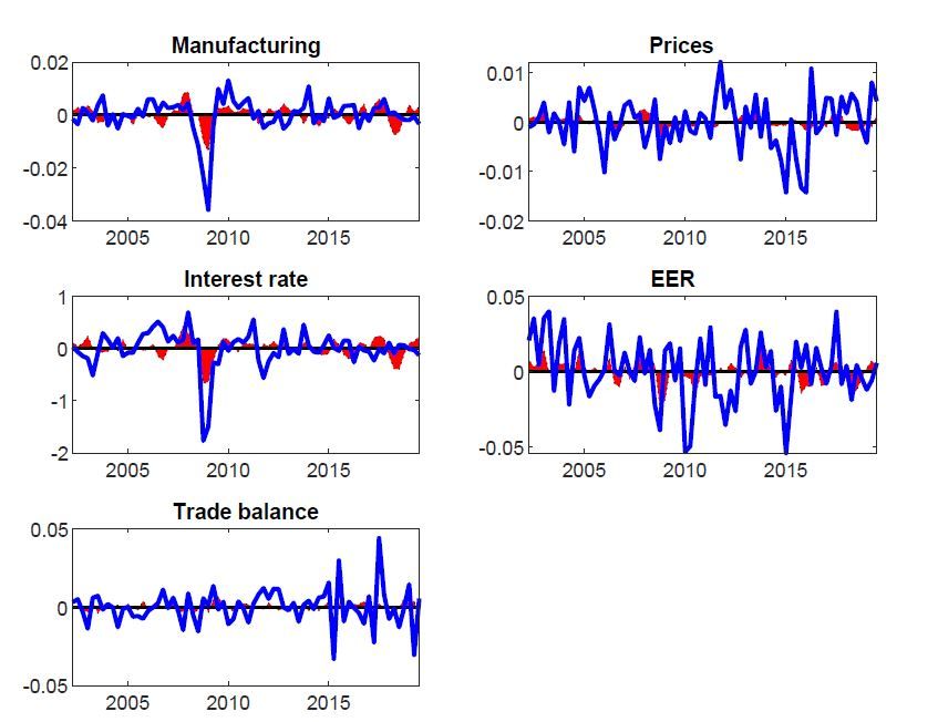
Historical decomposition. To assess the contribution of TPU shocks to the total
forecast error in each point in time, the historical decomposition of each EA variable is
plotted in Figure 3. Consistently with the impulse response functions and the forecast
error variance decomposition, TPU shocks play an important role in explaining the
volatility of the Euro EER during the Great Recession and over the last three years
when the US-China trade war has significantly intensified. Non-negligible support to
the Euro EER deviations is provided by TPU shocks even in the first part of the 2000s.
The same story can be told for the EA prices, although the contribution of TPU shocks
is smaller in this case. The GDP, interest rate and, to a much weaker extent, the trade
balance show interesting reactions over the period of the Great Recession and of trade
war tightening, but no significant provision is given during the other years.5
5
In Appendix, in Figure A1, we also plot the TPU shock series over the sample period.
14Figure 4: Contribution of TPU shocks to EA variables - historical decomposition
The recent trade tensions follow a gradual rise in protectionism. The number of
new sovereign measures restricting global trade has increased over the past decade,
while there have been relatively fewer measures favouring trade liberalization. For EA
countries, the number of harmful measures implemented or announced by its trading
partners has also been on the rise, potentially increasing trade costs for exporters and
businesses.
3.2 Alternative specifications
Tariff volatility. In the second specification of the model we check the responses of
the EA economy on the trade policy uncertainty shocks by replacing the TPU index
with the tariff volatility index. Similar to the TPU index, the tariff volatility exhibits
upswings of tariff uncertainty in periods of uncertainty in trade policies (Figure 5).
15Again, it is clearly evident that in the recent years the onset of the US-China trade
war has pushed the tariff volatility index above its historical median.
Figure 5: Tariff volatility index
Source: Caldara et al. (2020)
In this case the identification strategy of the model stays the same as in the baseline
case.6 The results of the model with tariff volatility offer similar conclusions as in the
baseline model. Figure 6 shows the median impulse response functions with the 68%
credible interval of the main EA macroeconomic variables to a tariff volatility shock.
As in the baseline model, the responses of the GDP and the interest rate to a tariff
volatility shock are stronger but less persistent in comparison to the responses of the
Euro EER and prices. Considering the alternative specification of the model by using
the tariff volatility index variable we are ale to produce similar results to the baseline
model and thus confirm the conclusions made by Caggiano et al. (2020) with respect
to the effects of uncertainty shocks on the nominal and real variables.
6
We follow the sign restriction matrix of the identified shocks from the Table 1.
16Figure 6: Impulse response functions of the EA variables to tariff volatility shocks
As in the baseline model, we compute the forecast error variance decomposition for
the model with tariff volatility (see Table A1 in the Appendix) and assess the contri-
bution of tariff volatility shocks to the total forecast error in each point in time with
the historical decomposition of each EA variable (see Figure A2 in the Appendix).
To test the informational content of the variables employed as proxies for trade policy
uncertainty, i.e. the news-based index of aggregate TPU and the tariff volatility in-
dex, we run the Granger-causality test based on bivariate VAR(4). On one hand, we
find that there are no evidence the news-based index of aggregate TPU to be Granger-
caused by the tariff volatility index (p-value = 0.86). On the other hand, the outcomes
suggest that we can reject the null hypothesis aggregate TPU does not Granger-cause
17the tariff volatility index (p-value = 0.00).
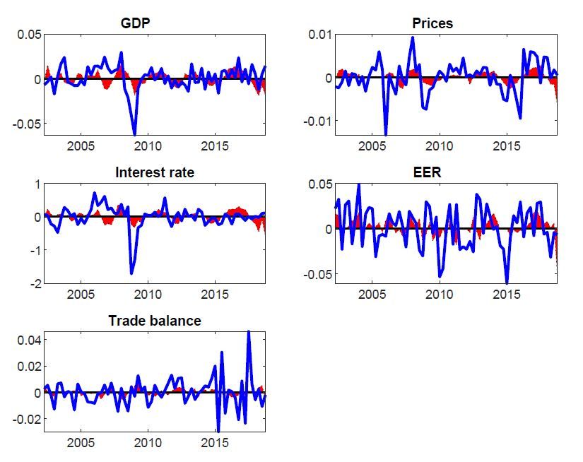
Manufacturing. We provide an additional specification of an alternative model that
considers manufacturing sector as the GDP proxy of the model. We maintain the same
identification procedure even for this specification. Again, we are able to produce ro-
bust results with the manufacturing model setting as the impulse response functions of
the EA macroeconomic variables show statistical significant responses to trade policy
uncertainty shocks (Figure 7).
Figure 7: Impulse response functions of the EA variables to TPU shocks - manufac-
turing.
We also compute the forecast error variance decomposition, that shows variation in
EA macroeconomic variables is due to the TPU shocks (see Table A2 in the Appendix).
Based on this, the contribution of TPU shocks to the total forecast error in each point
18in time, the historical decomposition of each EA variable plotted in Figure A3 in
the Appendix shows that the TPU shocks play an important role in explaining the
volatility of the macroeconomic EA variables.
4 Conclusions
Based on a number of developments in the global geo-political environment, the role of
the (trade) policy uncertainty raised discussions amongst researchers. The Brexit vote,
the height of the sovereign debt crisis in Europe and the outbreak of the US-China
trade war are one of the most important factors that have shaped the economic activ-
ities in recent years. In this paper we analyse the response of the EA business cycle
to the trade policy uncertainty shocks by estimating a number of structural shocks,
which are identified with a minimum set of sign restrictions in a Bayesian VAR model
setting.
The empirical results suggest that TPU shocks do have significant effects on the EA
economy, especially on prices and mostly on the Euro EER in the long-term. Output
and interest are also affected but their responses are sharper but last only for a couple
of quarters. To confirm our findings from the baseline model, we set up alternative
specifications. In the first one, we replace the TPU index with a different measure,
the tariff volatility. In the second one, we use manufacturing as a proxy for GDP.
Both alternatives are robust. Moreover, we also show that TPU shocks have a non-
homogeneous magnitude on the real economy, according to the sector that we consider.
19References
1. Bachmann, R., Elstner, S., & Sims, E.R. (2013). Uncertainty and Economic
Activity: Evidence from Business Survey Data. American Economic Journal:
Macroeconomics, 5(2), 217-249.
2. Baker, S.R., Bloom, N., & Davis, S.J. (2016). Measuring Economic Policy Un-
certainty. Quarterly Journal of Economics, 131(4), 1593-1636.
3. Barro, R.J., & King, R.G. (1984). Time-Separable Preferences and Intertemporal-
Substitution Models of Business Cycles. Quarterly Journal of Economics, 99(4),
817-839.
4. Basu, S., & Bundick, B. (2017). Uncertainty Shocks in a Model of Effective
Demand. Econometrica, 85(3), 937-958.
5. Bjørnland, H., & Leitemo, K. (2010). Identifying the Interdependence between
US Monetary Policy and the Stock Market. Journal of Monetary Economics,
56(2), 275-282.
6. Bloom, N. (2009). The Impact of Uncertainty Shocks. Econometrica, 77(3),
623-685.
7. Caggiano, G., Castelnuovo, E., & Figueres, J.M. (2017). Economic Policy Un-
certainty and Unemployment in the United States: A Nonlinear Approach. Eco-
nomic Letters, 151(C), 31-34.
8. Caggiano, G., Castelnuovo, E., & Figueres, J.M. (2020). Economic Policy Un-
certainty Spillovers in Booms and Busts. Oxford Bulletin of Economics and
Statistics, 82(1), 125-155.
9. Caggiano, G., Castelnuovo, E., & Groshenny, N. (2014). Uncertainty Shocks and
Unemployment Dynamics: An Analysis of Post-WWII U.S. Recessions. Journal
of Monetary Economics, 67(C), 78-92.
2010. Caldara, D., Iacoviello, M., Molligo, P., Prestipino, A., & Raffo, A. (2020). The
Economic Effects of Trade Policy Uncertainty. Journal of Monetary Economics,
109(1), 38-59.
11. Canova, F., & De Nicoló, G. (2002). Monetary Disturbances Matter for Business
Fluctuations in the G-7. Journal of Monetary Economics, 49(6), 1131-1159.
12. Canova. F., & Paustian, M. (2011). Business cycle measurement with some
theory. Journal of Monetary Economics , 58(4), 345-361.
13. Colombo, V. (2013). Economic Policy Uncertainty in the US: Does it Matter for
the Euro Area? Economic Letters, 121(1), 39-42.
14. Crowley, M., Meng, N., & Song, H. (2018). Tariff Scares: Trade Policy Uncer-
tainty and Foreign Market Entry by Chinese Firms. Journal of International
Economics, 114, 96-115.
15. Ebeke, C., & Siminitz, J. (2018). Trade Uncertainty and Investment in the Euro
Area. IMF Working Paper WP/18/281.
16. Faust, J. (1998). The Robustness of Identified VAR Conclusions about Money.
Carnegie-Rochester Conference Series on Public Policy,, 49(1), 207-244.
17. Fernández-Villaverde, J., Guerrón-Quintana, P., Kuester, K., & Rubio-Ramı́rez,
J. (2015). Fiscal Volatility Shocks and Economic Activity. American Economic
Review, 105(11), 3352–3384.
18. Fry, R., & Pagan, A. (2011). Sign Restrictions in Structural Vector Autoregres-
sions: A Critical Review. Journal of Economic Literature, 49(4), 938-960.
19. Furlanetto, F., Ravazzolo, F., & Sarferaz, S. (2019). Identification of Financial
Factors in Economic Fluctuations. Economic Journal, 129(617), 311-337.
20. Handley, K. (2014). Exporting Under Trade Policy Uncertainty: Theory and
Evidence. Journal of International Economics, 94(1), 50-66.
2121. Handley, K., & Limão, N. (2017). Policy Uncertainty, Trade, and Welfare: The-
ory and Evidence for China and the United States. American Economic Review,
107(9), 2731–2783.
22. Hassan, T.A., Hollander, S., van Lent, L., & Tahoun, A. (2019). Firm-Level Po-
litical Risk: Measurement and Effects. Quarterly Journal of Economics, 134(4),
2135–2202.
23. Jaimovich, N., & Rebelo, S. (2009). Can News about the Future Drive the
Business Cycle? American Economic Review, 99(4), 1097-1118.
24. Jurado, K., Ludvigson, S.C., & Ng, S. (2015). Measuring Uncertainty. American
Economic Review, 105(3), 1177-1216.
25. Kamber, G., Karagedikli, Ö., Ryan, M., & Vehbi, T. (2016). International Spill-
Overs of Uncertainty Shocks: Evidence from a FAVAR. CAMA Working Paper
61/2016 .
26. Leduc, S., & Liu, Z. (2016). Uncertainty Shocks are Aggregate Demand Shocks.
Journal of Monetary Economics, 82(C), 20-35.
27. Nodari, G. (2014). Financial Regulation Policy Uncertainty and Credit Spreads
in the US. Journal of Macroeconomics, 41(C), 122–132.
28. Peersman, G. (2005). What Caused the Early Millennium Slowdown? Evidence
Based on Vector Autoregressions. Journal of Applied Econometrics, 20(2), 185-
207.
29. Peersman, G., & Straub, R. (2006). Putting the New Keynesian model to a test.
IMF working paper 06/135.
30. Rice, J. (2020). Economic Policy Uncertainty in Small Open Economies, a Case
Study of Ireland. Central Bank of Ireland Research Technical Paper Vol. 2020,
No. 1.
2231. Rigobon, R., & Sack, B. (2003). Measuring the Reaction of Monetary Policy to
the Stock Market. Quarterly Journal of Economics, 118(2), 639–669.
32. Schnabl, G. (2008). Exchange Rate Volatility and Growth in Small Open Economies
at the EMU Periphery. Economic Systems, 32(1), 70-91.
33. Sims, C., Stock, J., & Watson, M. (1990). Inference in Linear Time Series Models
with some Unit Roots. Econometrica, 58(1), 113–144.
34. Sims, C., & Uhlig, B. (1991). Understanding Unit Rooters: A Helicopter Tour.
Econometrica, 59(6), 1591-1599.
35. Steinberg, J.B. (2019). Brexit and the Macroeconomic Impact of Trade Policy
Uncertainty. Journal of International Economics, 117(C), 175-195.
36. Uhlig, B. (2005). What are the Effects of Monetary Policy on Output? Results
from an Agnostic Identification Procedure. Journal of Monetary Economics,
52(2), 381–419.
23Appendix A
Figure A1: TPU shock over the sample period
Table A1: Forecast error variance decompositions of EA variables to selected shocks -
alternative model with tariff volatility
Trade Supply Monetary Global
uncertainty policy demand
Variable h = 5, h = 13 h = 5, h = 13 h = 5, h = 13 h = 5, h = 13
GDP 0.10, 0.06 0.23, 0.14 0.03, 0.06 0.17, 0.13
Prices 0.26, 0.14 0.11, 0.18 0.41, 0.41 0.03, 0.13
Interest rate 0.13, 0.12 0.21, 0.20 0.02, 0.08 0.08, 0.10
Euro EER 0.14, 0.23 0.04, 0.03 0.18, 0.20 0.09, 0.10
Trade balance 0.02, 0.04 0.37, 0.25 0.19, 0.33 0.37, 0.27
iFigure A2: Contribution of TPU shocks to EA variables - historical decomposition
(tariff volatility)
Table A2: Forecast error variance decompositions of EA variables to selected shocks -
alternative model with manufacturing
Trade Supply Monetary Global
uncertainty policy demand
Variable h = 5, h = 13 h = 5, h = 13 h = 5, h = 13 h = 5, h = 13
Manufacturing 0.16, 0.12 0.15, 0.12 0.01, 0.02 0.28, 0.18
Prices 0.24, 0.12 0.32, 0.47 0.34, 0.23 0.03, 0.01
Interest rate 0.18, 0.12 0.14, 0.12 0.09, 0.17 0.18, 0.18
Euro EER 0.10, 0.21 0.06, 0.05 0.14, 0.15 0.10, 0.11
Trade balance 0.04, 0.05 0.53, 0.48 0.14, 0.17 0.20, 0.13
iiFigure A3: Contribution of TPU shocks to EA variables - historical decomposition
(manufacturing)
iiiAppendix B
We report here details of the estimation procedure. We closely follow Furlanetto et al.
(2019).
We rewrite the VAR model in (1) in its compact way:
Y = BX + U (3)
where Y = [y1 . . . yT ]′ , B = [CB1 . . . Bp ]′ , U = [u1 . . . uT ]′ , and
1 y0′ ··· y−p
′
.. .. .. ..
X=
. . . .
(4)
1 yT′ −1 ··· yT′ −p
The compact VAR model presented in (3) can be rewritten in its vectorized form:
y = (IN ⊗ X) (5)
where vec() stands for columnwise vectorization, y = vec(Y ), β = vec(B), and u =
vec(U ). We assume error term to be normally distributed with zero mean and variance-
covariance matrix equal to Σ ⊗ IT .
The likelihood function in B and Σ is
T 1 1
L(B, Σ) ∝ |Σ|− 2 exp{− (β − β̂)′ (Σ−1 ⊗ X ′ X)(β − β̂)} exp{− tr(Σ−1 S)} (6)
2 2
where S = ((Y −X B̂)′ (Y −X B̂)) and β̂ = vec(B̂) with B̂ = (X ′ X)−1 X ′ Y . We assume
diffuse priors so that the information in the likelihood is dominant and these priors
lead to a Normal-Wishart posterior. In more detail, we use a diffuse prior for β and
ivn+1
Σ that is proportional to |Σ|− 2 . The posterior is then
T +n+1 1 1
p = (B, Σ|Y, X) ∝ |Σ|− 2 exp{− (β − β̂)′ (Σ−1 ⊗ X ′ X)(β − β̂)} exp{− tr(Σ−1 S)}
2 2
(7)
The posterior in (3) is the product of a normal distribution for β conditional on Σ and
an inverted Wishart distribution for Σ (see, e.g. Kadiyala and Karlsson, 1997 for the
proof). We then draw β conditional on Σ from
β|Σ, Y, X ∼ N (β̂, Σ ⊗ (X ′ X)−1 ) (8)
and Σ from
Σ|Y, X ∼ IW (S, v) (9)
where v = (T − n) ∗ (p − 1) and N representing the normal distribution and IW the
inverted Wishart distribution.
vYou can also read