Uncertainty in marine weather routing
←
→
Page content transcription
If your browser does not render page correctly, please read the page content below
Uncertainty in marine weather routing
                                                     Thomas Dickson            Helen Farr              David Sear
arXiv:1901.03840v1 [math.NA] 12 Jan 2019

                                                                          James I R Blake
                                                                          January 15, 2019

                                           1    Introduction
                                                                                 Abstract
                                                    Weather routing methods are essential for planning routes for commer-
                                                cial shipping and recreational craft. This paper provides a methodology
                                                for quantifying the significance of numerical error and performance model
                                                uncertainty on the predictions returned from a weather routing algorithm.
                                                The numerical error of the routing algorithm is estimated by solving the
                                                optimum path over different discretizations of the environment. The un-
                                                certainty associated with the performance model is linearly varied in order
                                                to quantify its significance. The methodology is applied to a sailing craft
                                                routing problem: the prediction of the voyaging time for an ethnographic
                                                voyaging canoe across long distance voyages in Polynesia. We find that
                                                the average numerical error is 0.396%, corresponding to 1.05 hours for
                                                an average voyage length of 266.40 hours. An uncertainty level of 2.5%
                                                in the performance model is seen to correspond to a standard deviation
                                                of ±2.41 − 3.08% of the voyaging time. These results illustrate the sig-
                                                nificance of considering the influence of numerical error and performance
                                                uncertainty when performing a weather routing study.
                                               Marine weather route modelling identifies the minimum time path between
                                           two locations given the performance model and the weather that is expected
                                           on a given route. Route modelling can be used within the design process for
                                           new designs or to provide routes for existing marine craft. When applied op-
                                           erationally, weather routing is essential for improving the safety of mariners at
                                           sea through identifying routes which minimise fuel costs, risk of harm or time.
                                               Quantifying the significance of uncertainty in the weather routing process
                                           allows the credibility of the predictions to be quantified, managing the expecta-
                                           tions of the operators with regards to the accuracy of the supplied route. Key
                                           sources of uncertainty are the weather data, the accuracy of the performance
                                           model and the numerical error in the solution of the shortest path algorithm.
                                           However, research has not investigated the quantification of the numerical er-
                                           ror of the routing algorithm or the impact of uncertainty in the performance
                                           model. The increasing availability of high performance computing and associ-
                                           ated improvement of programming languages allows previously computationally
                                           intractable problems to be simulated.

                                                                                    1
This paper introduces a methodology for quantifying the significance of nu-
merical error and performance uncertainty in a marine weather routing study.
Initially the numerical error of the shortest path algorithm will be quantified
through varying the discretization of the environment. The influence of uncer-
tainty of the performance is estimated through varying the performance linearly
about the original performance model.
     A marine weather routing problem with a high level of uncertainty is the
modelling of ethnographic voyaging canoes completing colonisation voyages across
Polynesia. This problem involves predicting the voyaging time of a sailing craft
over a given route for a range of weather conditions, a typical design problem.
It is possible to model the performance of any marine craft as a function of wind
and wave conditions, allowed this method to be applied to any marine craft.

1.1    Literature review
This review will discuss the literature on sailing craft performance prediction and
weather routing algorithms. The weather routing process predicts the optimum
route for a sailing craft to take between two points. The method considers the
performance model of the sailing craft, the shortest path algorithm and the
environmental data used to identify the optimum path.
    The performance of a sailing craft is determined by the balance of the driving
force generated by the wind passing over the sail against the resistance of the hull
and appendages. The wind passing over the sail also generates a heeling moment
which is balanced against the righting moment of the hull. The interaction of
these key force balances and the additional moments determine the speed and
heel angle of the sailing yacht (Philpott et al., 1993).
    Static and dynamic velocity prediction programs (VPPs) are used to model
the performance of a sailing craft. Static VPPs predict the conditions at which
the forces and moments acting on a sailing craft are balanced (Philpott et al.,
1993). Dynamic VPPs evaluate the forces acting on the sailing craft over a
series of time steps, within the context of a short race (Philpott et al., 2004).
Static VPPs require less information than dynamic VPPs on the design of a
sailing craft to provide performance predictions but are considered to be less
accurate as a result.
    The first research into solving the sailing craft route optimisation problem
used a recursive dynamic programming formulation which divided the domain
into nodes over which the shortest path was calculated Allsopp (1998). Different
wind models Philpott et al. (2004); Dalang et al. (2015) or race strategy and
opponent models Spenkuch (2014); Tagliaferri and Viola (2017) have been used
to improve the accuracy of sailing routing models.
    The influence of different methods of modelling the ability for a sailing craft
to sail upwind has been explored Stelzer and Pröll (2008) along with modelling
the time taken to complete course changes Ladany and Levi (2017). Sailing
craft race modelling has typically minimised either the time taken to complete
a course Ferretti and Festa (2018), risk of losing to an opponent Tagliaferri
et al. (2014); Spenkuch (2014) or reliability (Dickson et al., 2018). However, the

                                         2
majority of sailing craft routing research only applies to a short course sailed
over a small spatial and temporal domain.
The long course modelling problem can be characterised through its consid-
eration of larger spatial and temporal domains over which the shortest path is
solved. Typical drawbacks of short course routing methods involve their require-
ment for a predictable wind field and the requirement for the entire course to be
modelled as being flat with respect to the curvature of the earth. The haversine
formula becomes accurate at distances longer than 1 nm (Allsopp, 1998), this
provides an indication at the crossover between short and long course routing
methods.
The marine weather routing literature has developed a range of different
shortest path algorithms. The different approaches were classified into calculus
of variations, grid based approaches and evolutionary optimisation (Walther
et al., 2016). A time dependent approach based on the calculus of variations
solved the shortest path problem through identifying the shortest path to take
through considering a series of fronts reached within incremental time steps
(Bijlsma, 1975). Forward dynamic programming approaches involve recursively
solving the shortest path over a grid of locations generated along the great circle
line between the start and finish locations (Allsopp, 1998). This approach can
be two dimensional or three dimensional considering how the variables such
as time and fuel cost are optimised Hagiwara and Spaans (1987). A claimed
improvement is to use a floating grid system which updates potential locations
every time step (Lin et al., 2013). These grids can be generated based off local
wind conditions (Tagliaferri and Viola, 2017), although this approach would be
challenging for larger spatio-temporal domains as found in long course routing.
Another route modelling approach has involved generating candidate routes
using biased Rapidly exploring Random Trees which solve for the minimum
energy path using the A∗ algorithm (Rao and Williams, 2009). A multi objective
genetic algorithm has been applied to solve for the optimum path considering
multiple safety and fuel constraints (Hinnenthal, 2008). An improvement came
with the implementation of a fuzzy logic model to model the performance of a
sail driven vessel (Marie and Courteille, 2014).
A method of iteratively aggregating the shortest path over multiple weather
scenarios has been introduced (Allsopp, 1998). The approach of using ensemble
weather scenarios has been shown to be more accurate than single scenarios
with application to marine weather routing (Skoglund et al., 2015). Multiple
algorithms and objective functions have been implemented and applied to the
marine weather routing problem. To the authors knowledge there has been no
study of how uncertainties within the solution algorithm and objective function
influence the confidence that may be had in the final result.
1.2 Uncertainty analysis
Uncertainty analysis is the process of quantifing how likely certain states of a
system are given a lack of knowledge on how certain parts of the system oper-
ate. The choice of how to categorize and thus simulate uncertainty is significant
3in the scientific modelling process (Der Kiureghian and Ditlevsen, 2007). In
the marine environment it is possible to classify uncertainty as being aleatory
uncertainty or epistemic uncertainty (Bitner-Gregersen et al., 2014). Aleatory
uncertainty is the inherent randomness in a particular parameter, it is not pos-
sible to reduce this. Epistemic uncertainty is knowledge based, it is possible to
reduce this quantity through collecting more information on the process in ques-
tion. Epistemic uncertainty can be broken down into data uncertainty, statis-
tical uncertainty, model uncertainty and climate uncertainty. Data uncertainty
is associated with the error associated with collecting data from experiment or
model. Statistical uncertainty is a consequence of not obtaining enough data
to model a given phenomenon. Climate uncertainty addresses the ability for
the climate variables over a given spatial-temporal domain to be representa-
tive given the nature of the weather and climate change (Bitner-Gregersen and
Hagen, 1990).
The weather has been described as a chaotic process (Lorenz, 1963). The
chaotic nature of the weather limits the ability to utilise numerical models to
predict into the future or to model what occured in the past. A chaotic system
can be thought of as one where the present state determines the future state,
but the approximate present state doesn’t determine the approximate future.
The use of ensemble weather scenarios generated using different intial conditions
attempts to mitigate the associated uncertainty with weather forecasts and re-
analysis data (Slingo and Palmer, 2011). Given that the weather is a chaotic
process, it is likely that any solution process for the shortest path sequential
decision making process may identify one or more stable solutions. Currently
the simplest method of simulating weather uncertainty is through using past
weather data.
The error in a scientific model is the accuracy at which it estimates a real
system. The key source of error is the ability for the shortest path algorithm
to identify the optimal path based on the discretization of the environment.
Typical discretization error calculation methods require grids of significantly
different sizes to be solved for a given set of initial conditions (Roache, 1997).
Through examining the rate of convergence of solutions from different grids it
is possible to extrapolate the solution for an infinite discretization.
2 Method
Figure 1 shows the method used in this research. The initial conditions such as
the route and environmental conditions are specified. A suitable routing algo-
rithm is identified and implemented. The numerical error is then estimated and
the influence of performance uncertainty is modelled. The method is concluded
with an analysis of the impact of performance uncertainty and numerical error
on the interpretation of the final set of voyaging time results.
4Initial conditions
Routing algorithm
Numerical error
Performance
uncertainty
Uncertainty
quantification
Figure 1: Method used to quantify uncertainty in marine weather routing.
2.1 Routing model
This paper uses the Dynamic Programming (DP) algorithm as applied to long
distance sailing craft in (Allsopp, 1998), the simplicity of this algorithm means
that the source of uncertainty lies in the discretization of the domain over which
the shortest path is solved.
We consider a large domain on the Earths surface over which the modelled
sailing craft could hypothetically sail. This domain is discretized into an equal
number of locations both in parallel and perpendicular to the Great Circle drawn
between the start and finish locations. The distance between each location is
controlled through defining the maximum distance between nodes, dn . dn can
be controlled seperately as the grid height or grid width, as seen in Figure 2, for
this research it is set as being equal. This generates a grid of nodes with equal
numbers of ranks as well as nodes within each rank.
For the position at any given node i the travel time between nodes i and
a node on the next rank j along the arc (i, j) starting at time t is carc (i, j, t).
The cost function, carc (i, j, t), provides an estimate of the time taken for a
sailing craft to sail between two points given the environmental conditions at
time t. An intial speed estimate is taken from interpolating the results of a
performance prediction analysis for the specific wind condition. This speed is
then modified in order to account for the wave conditions being experienced. A
final optimisation takes place to identify the optimum heading to sail between
the two points given the current the craft is exposed to. If it is not possible to
achieve a positive speed towards location i from location j then the speed will
be set to 0 returning an infinite travel time for that particular arc. It is possible
to penalise areas of the domain in this manner and identify combinations of
5Figure 2: Discretized domain along great circle line between voyage start and
finish.
initial conditions which are unable to return
The minimum time path is identified using a forward looking recursive al-
gorithm, described in Equation 1. f ∗ (i, t) is the time taken for the optimal se-
quence of decisions from the node-time pair (i, t) to the finish node and j ∗ (i, t) is
the successor of i on the optimal path when in state t. Through solving j ∗ (i, t)
within f ∗ (i, t) it’s possible to solve for the shortest path. Γi is the set of all
nodes on the graph. The algorithm iterates from the start node to the finish
node and updates each node in between with the earliest time that it can be
reached.
(
∗ 0, i = nf inish
f (i, t) =
minj∈Γi [carc (i, j, t) + f ∗ (j, t + carc (i, j, t))], otherwise (1)
j ∗ (i, j) = arg min [carc (i, j, t) + f ∗ (j, t + carc (i, j, t))], i 6= nf inish
j∈Γi
2.2 Uncertainty simulation
The primary sources of uncertainty in sailing craft route modelling lie in the
accuracy of the solution algorithm, the performance model of the sailing craft
and the weather. This section introduces the method used to investigate the
solution accuracy of the algorithm and the influence of performance uncertainty
of a sailing craft.
The discretization of the environment is the primary source of numerical un-
certainty in the solution algorithm. The key parameter determining the fidelity
of the simulation is the distance between nodes dn . We are interested in the
significance of this parameter on the results on any given routing analysis. In
6order to consider the influence of the discretization of the domain on sailing
craft routing results the lower limit of dn must be identified which will allow
two coarser grid sizes to be chosen.
The lower limit of dn is selected based on the minimum distance at which the
cost function retains accuracy. Influencing factors include the discretization of
the sailing domain and the spatial and temporal resolution of the weather data
used. For example, if the time taken to travel between two locations is greater
than the temporal resolution of the weather dataset then there are changes in
weather conditions which are not being modelled.
The weather data used is from the ERA20 climate model has a spatial res-
olution of 125 km and a temporal resolution of 3 hours (Poli et al., 2016). The
weather data is linearly intepolated to the discretization of the nodes in the
environment. If the distance between nodes is much larger than the original
spatial discretization of the weather data then the change in the weather con-
ditions will not be fully modelled. The voyaging time is used to look up the
closest weather data time step.
The accuracy of the performance model is limited to certain scales, conse-
quently it may not make physical sense to apply such a model below a certain
length of time or distance. Despite this, a quantification of the numerical so-
lution algorithm is still required in order to identify whether the shortest path
solution is stable. One index used to quantify numerical uncertainty in CFD is
the grid convergence index (GCI) (Roache, 1997; Ghia et al., 2008) which has
only recently been applied to the sailing craft routing problem (Dickson et al.,
2018).
The method of numerically quantifying error using the Grid Convergence
Index (GCI) is fully described in Ghia et al. (2008). It involves the solution of the
algorithm over multiple discretizations of the environment which exponentially
increase in detail. The grid height, h, is the measurement unit of grid size and
is calculated using Equation 2. ∆Ai is the size of the ith cell and N is the
total number of the cells used for computation. The solution trend from the
three distinct grid sizes is extrapolated towards h → 0 where the extrapolated
solution is used to estimate the associated discretization error.
h1 XN i
h= (∆Ai ) (2)
N i=1
We wish to quantify whether uncertainty surrounding the performance mod-
elling of a sailing craft is significant within the context of sailing craft route
modelling. To begin the process the performance model is varied linearly about
its original performance value. Each generated performance model is known as
Punc , where unc is the percentage that the original performance is varied by.
Algorithm 1 describes the uncertainty simulation routine for a specific route
at a specific time. It shows how the shortest path is simulated for each dn pa-
rameter and range of Punc values at a start time t for a given route. The number
of start times and uncertain performances to be simulated is dependent on the
7computational resources available. The code for this method was implemented
in the programming language Julia (Bezanson et al., 2017).
Algorithm 1 Route modelling uncertainty simulation routine for a specific
start time t and route.
1: procedure Routing uncertainty simulation
2: for dn in [h1 , h2 , h3 ] do
3: Generate discretized environment
4: Spatially interpolate wind, wave and current data for each node
5: for Punc in[50%, ..., 150%] × Pprediction do
6: Vt,dn ,unc ← Shortest path(t, dn , Punc )
3 Application
The uncertainty route modelling analysis procedure is applied to quantifying
the performance of Polynesian voyaging canoes, an application with previously
irreducible levels of uncertainty. Modelling the voyaging time for ethographic
voyaging craft to complete specific routes will assist understanding how it was
possible for Polynesia to be colonised, one of Pacific archaeology’s greatest unan-
swered questions (Irwin and Flay, 2015). Of interest is the influence of the
ENSO oscillation, a key weather phenomenon in the Pacific, on the voyaging
time (Montenegro et al., 2016). One voyaging route of interest is between Upolu
and Moorea. Through simulating the influence of performance uncertainty on
the voyaging time for a colonisation voyage it will be possible to quantify the
influence of seafaring technology on the rate of the colonisation of Polynesia. At
the heart of this problem is the solution of a marine weather routing algorithm
with a prior requirement to simulate uncertainty.
The shortest path between Tongatapu and Atiu was estimated for a range
of different grid sizes, performances and start times. The results from this
series of simulations can be used to estimate the difficulty of making the voyage
between these two locations using prehistoric seafaring technology. Twenty
different performances were generated linearly varying from −50% to +50% of
the original performance model. Voyages were started every 72 hours from the
1st January to the 31st December. 1985 is used to provide weather data for a
medium ENSO, an important condition in the context of the study.
To quantify the efficacy of later voyaging canoe designs, performance data
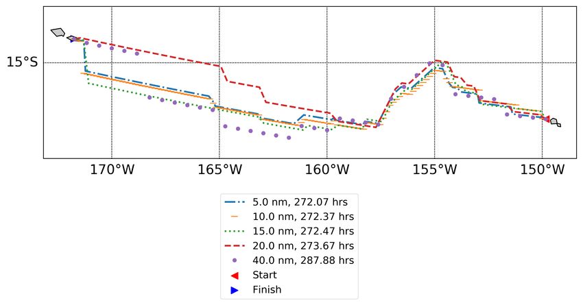
from an outrigger canoe was used (Boeck et al., 2012). The cost function for
this craft interpolates the performance from the polar performance diagram,
seen in Figure 3a. An example of how the performance is varied for a specific
wind condition is shown in Figure 3b. The wind and wave reanalysis data was
downloaded for the year 1982 from the ECMWF ERA20 model Poli et al. (2016).
The current data used was sourced from (Bonjean and Lagerloef, 2002).
8(a) Vs as a function of true wind speed and (b) Boat speed, Vs , varied 10% about the
direction for the ethnographic sailing craft original performance for a wind speed of 10
Boeck et al. (2012). kts.
Figure 3: Performance of marine vessel used in study.
3.1 Numerical uncertainty
3.1.1 Illustration of simulation convergence
The numerical error in the routing algorithm is a function of the discretization
of the domain, parameterised by the grid width, dn . Figure 4 illustrates the
predicted routes between Tongatapu and Atiu where dn was reduced in stages
between 40.0 to 5 nm. It can be seen that as the fidelity of the simulation
increases, the voyaging time, Vt , reduces.
A convergence plot of Vt as a function of dn is shown in Figure 5. For the
specific initial conditions the relationship is that as dn reduces, so too does Vt .
It can be seen that there is a significant change in relationship between the
results for dn = 40, 20 and dn = 15, 10, 5 nm and Vt . This could be due to
the grid discretization becoming significantly finer than the resolution of the
original wind and wave data.
The extrapolated Vt , GCI and order of convergence for three combination of
heights is included in Table 1. The extrapolated Vt value is where the predicted
Vt for the specified heights is extrapolated to dn = 0. For dn = 10.0, 15.0, 20.0
we see there is a low associated GCI as it looks as if the results are converging
rapidly. However, we see that for both dn = 5.0, 10.0, 15.0 nm the GCI increases
by an order of magnitude as Vt reduces. This indicates that as the accuracy
of the simulation improves the application of GCI becomes meaningful. How-
ever, there is a large computational cost associated with finer simulations which
prohibits the number of simulations required to explore uncertainty in voyaging
time. These results show that the GCI calculation method for estimating nu-
9Figure 4: Routes between Upolu and Moorea starting at 00:00 GMT on the 1st
January 1985 solved over several different grid widths.
Figure 5: Voyaging time, Vt , as a function of grid width for voyages between
Upolu and Moorea starting at 00:00 GMT on the 1st January 1985.
merical error must be applied in a manner considering the physical implication
of the parameters but also the computational run time of the simulations.
The selection of dn is a compromise between simulation accuracy and com-
putational run time. Simulation accuracy is determined by the smallest and the
largest scales that the cost function can be applied to. The smallest scale is
determined by the haversine formula which has significant levels of error for dis-
tances below 1 nm. The largest scale is determined by the rate at which spatio-
temporal environmental data becomes available. Parallel computing provides
10dn Vt (hrs) GCI OOC
5.0, 10.0, 15.0 274.00 0.0014577 2.25
10.0, 15.0, 20.0 272.49 0.0000955 4.34
15.0, 20.0, 40.0 272.64 0.0012429 2.59
Table 1: Calculation of extrapolated Vt , GCI and order of convergence.
significantly more resources than available previously allowing an increase in the
number of different initial conditions that are required to be simulated. However,
there are still large costs associated with the finer simulations at dn = 2.5, 5.
Figure 5 illustrates that as dn is reduced significantly below the spatial dis-
tribution of weather data there is a step change in the solution. The dn also
influences the rate at which new weather data is retrieved and processed. If the
journey time for a particular arc between two nodes lasts longer than the time
between weather conditions being updated then the solution is being solved over
incomplete information. The desire for accuracy must be balanced against com-
putational limitations. There is a cubic relation between the computational run
time and fidelity of the simulation. From this set of initial simulations it may be
proposed that the dn = 10.0, 15.0, 20.0 nm provide a collection of heights which
balance the requirement for accuracy against computational run time.
3.1.2 Numerical error of voyaging simulations
Of interest is the average numerical error for the group of simulations being run.
The numerical error must be calculated for each set of initial conditions, but
knowledge of the average error will give a sense of the degree of confidence we
might have. We are interested in what is the most likely amount of numerical
error which might exist.
The order of convergence, GCI value and extrapolated voyaging time were
calculated for the times generated as a function of the different grid sizes of 10, 15
and 20 nm. The order of convergence measures the rate at which the difference
between the magitude of each result changes as a function of the change of the
grid width. 95.66% of the remaining results had an order of convergence greater
than 1.0, a necessary requirement in order to extrapolate the result to a grid
width of approximately 0.
The lack of convergence is due to the solution of a shortest path algorithm,
a sequential decision making problem, over a chaotic environment. For those
remaining results it is possible to investigate the lack of convergence through
running simulations at reduced grid widths. For now, the use of the numer-
ical error reduction procedure helps identifying which combinations of initial
conditions result in complex behaviour requiring more analysis.
The relationship between Vt and GCI is shown in Figure 6. It can be seen
that there is no relationship between Vt and GCI. This can be explained as
the same number of calculations are being performed over each grid size. It can
11be seen that large deviations from the mean Vt are associated with large GCI
values. This indicates sets of initial conditions where more analysis is required in
order to arrive at credible predictions. The relationship between the converged
results and GCI values estimates an average of 0.396%Vt error associated with
the whole group of converged voyaging time predictions. This is approximately
1.05 hrs for the mean voyaging time of 266.40 hrs.
Figure 6: Relationship between GCI index and voyaging time.
3.2 Performance uncertainty
The ethnographic voyaging canoe acts as an example of a typical marine craft
design problem, albeit one with large levels of uncertainty. Voyages between
Tongatapu and Atiu were started every 6 hours from the 1st January 1985
to the 31st December 1985. The performance model was varied for 21 steps
between 50% and 150% of the original performance. Simulations were solved
over a grid size of dn = 10 nm. Significant variation in voyaging time can be
seen for any given performance and across all changes in performance, as seen
in Figure 7.
The mean voyaging time appears to be between 230 − 295 hours for the
unaltered performance with the variation being solely due to the range of en-
vironmental conditions. This illustrates that even if there was a high level of
confidence associated with the accuracy of the performance model the weather
conditions contribute signficantly to the variation of voyaging time.
Across the range of performance variation variation there is a large change
from a minimum voyaging time of 98.42 hours up to a maximum of 682.77
hours. A lack of confidence in the accuracy of the performance model increases
12Figure 7: Voyaging time as a function of the different variations of performance.
The standard deviation is illustrated using error bars.
the variation in voyaging time. The accuracy of the performance model must
be quantified before performing a routing study so it is possible to quantify the
realistic variation in voyaging time.
Of interest is the variance of the voyaging time as a function of the perfor-
mance variation. Understanding how as the varying of performance influences
the voyaging time indicates the degree of confidence that should be held in a
given voyaging result, given the confidence in the performance mode.
Figure 8 shows the relationship between performance variation and the voy-
aging time non-dimensionalised with respect to the original performance voy-
aging time for each start date. This illustrates how variations in performance
from the original performance significantly alter the expected voyaging time.
It can be seen that as the performance varies from the initial performance the
standard deviation of the voyaging time results increases. One key result is that
the magnitude of the reduction of voyaging time in response to performance
improvement is smaller than the magnitude of the increase of voyaging time in
response to performance reduction.
There is also a difference between the change in the standard deviation of
Vt for equivalent magnitude variations about the original performance. As the
performance decreases we see more significant reductions in speed and much
larger increases in standard deviation. As the performance increases the mag-
nitude between successive improvements decreases along with a reduction in
standard deviation. It can be seen that reductions in performance have more
significant negative impacts on voyaging time than equivalent improvements.
This non-linear response is due to the slower craft spending more time at sea
13Figure 8: Relationship between the voyaging time and change in performance.
The standard deviation is plotted as the error bars.
and consequently being exposed to more variation in the weather.
Figure 9 shows how the standard deviation of the voyaging time varies as
a function of the performance variation. The average numerical is overlaid to
provide an indication of how significant it may be when using the results of
this study. Figure 9 indicates that the contribution of performance uncertainty
is much larger than the numerical error of the algorithm. A variation in per-
formance of ±2.5% causes a standard deviation of 0.8 − 1.1%, equivalent to
2.13 − 2.93 hrs for the mean voyaging time of 266.40 hrs. As the variation from
the original performance increases to ±5% we see that the standard deviation
increases rapidly to 2.41 − 3.08%Vt , or, 6.42 − 8.21 hours. These results indicate
that uncertainty in the cost function describing the performance of a sailing
craft signficiantly change the estimated voyaging time of the shortest path.
The weather conditions are updated every 3 hours. The magnitude of the
numerical error and influence of low levels of performance uncertainty indicate
that it is possible for multiple changes in the weather to not be modelled. It
would be difficult to quantify the impact of this error on the ability for the
weather routing model to approximate the real situation.
14Figure 9: Relationship between performance variation and the standard devia-
tion of Vt,P100% .
4 Summary and conclusions
This paper has presented a method for evaluating the impact of numerical error
and performance variation in the voyaging time for a marine weather routing
problem. This method was applied to a typical design problem; the quantifi-
cation of the time taken for a sailing craft to complete a specific voyage given
uncertainty in its performance. The key results of this study can be summarised
as follows;
1. Variation in performance contributed significantly to the variation in voy-
aging time given the existing variation due to change in environmental
conditions.
2. The numerical error must be calculated for each set of initial conditions.
For this problem, 95.3% of all simulations converged with an average of
0.396% error, equivalent to 1.05 hours for an average voyage length of
266.40 hours.
3. Slower craft spend more time at sea they are exposed to more variance in
the weather conditions, likely contributing towards the non-linear response
of voyaging time to performance variation. This means that the uncer-
tainty in the performance model must be quantified to provide credibility
to voyaging simulations.
4. There is a non linear relationship between variation of performance and
voyaging time. The relationship between uncertainty and the standard
deviation of voyaging time increases sharply with variations of 2.5% in
performance being associated with standard deviations of ±2.41 − 3.08%
15about the mean voyaging time. The influence of uncertainty in the perfor-
mance model rapidly becomes more influential than the routing algorithm
numerical error,
5. The weather data used updates every 3 hours. The combination of nu-
merical error and uncertainty in performance model may mean that the
approximation of the shortest path is being calculated based off incom-
plete sets of weather data, or solved using more weather data than would
be encountered in practice.
This method of quantifying the numerical error of the solution algorithm
and performance uncertainty could be applied to other cases involving marine
vessels such as cargo ships. This would allow an understanding of the maximum
level of accuracy that could be achieved within commerical practice. Another
investigation could be into the uncertainty levels associated with the recorded
reanalysis weather data used and how this might influence the result.
Through applying an uncertainty analysis method to the marine weather
routing problem we have shown that the influence of performance uncertainty is
much larger than any uncertainty associated with the shortest path algorithm
used. To provide more accurate routing the uncertainty associated with the
performance model used must be reduced.
Acknowledgements
Dr Gabriel Weymouth, Professor Dominic Hudson and Dr Blair Thornton for
discussion of methodology and results. Carlos Losada de la Lastra for extensive
comments on the text.
Funding sources
This work was funded by the Southampton Marine and Maritime Institute and
the University of Southampton.
References
A. B. Philpott, R. M. Sullivan, P. S. Jackson, Theory and Methodology Yacht
velocity prediction using mathematical programming, European Journal of
Operational Research 67 (1993) 13–24.
A. B. Philpott, S. G. Henderson, D. Teirney, A Simulation Model for Predicting
Yacht Match Race Outcomes, Operations Research 52 (2004) 1–16.
T. Allsopp, Stochastic Weather Routing for Sailing Yachts, Masters, The Uni-
versity of Auckland, 1998.
16R. C. Dalang, F. Dumas, S. Sardy, S. Morgenthaler, J. Vila, Stochastic optimiza-
tion of sailing trajectories in an upwind regatta, Journal of the Operational
Research Society 66 (2015) 807–821.
T. B. Spenkuch, UNIVERSITY OF SOUTHAMPTON A Bayesian Belief Net-
work Approach for Modelling Tactical Decision-Making in a Multiple Yacht
Race Simulator By (2014).
F. Tagliaferri, I. M. Viola, A real-time strategy-decision program for sailing
yacht races, Ocean Engineering 134 (2017) 129–139.
R. Stelzer, T. Pröll, Autonomous sailboat navigation for short course racing,
Robotics and Autonomous Systems 56 (2008) 604–614.
S. P. Ladany, O. Levi, Search for optimal sailing policy, European Journal of
Operational Research 260 (2017) 222–231.
R. Ferretti, A. Festa, A Hybrid control approach to the route planning problem
for sailing boats, Http://Arxiv.Org/Abs/1707.08103 (2018) 1–27.
F. Tagliaferri, A. B. Philpott, I. M. Viola, R. G. Flay, On risk attitude and
optimal yacht racing tactics, Ocean Engineering 90 (2014) 149–154.
T. Dickson, J. Blake, D. Sear, Reliability informed routing for Autonomous
Sailing Craft, in: S. Schillai, N. Townsend (Eds.), International Robotic
Sailing Conference, Southampton, 2018.
T. Allsopp, Stochastic Weather Routing for Sailing Yachts (1998) 110.
L. Walther, A. Rizvanolli, M. Wendebourg, C. Jahn, Modeling and Optimization
Algorithms in Ship Weather Routing, International Journal of e-Navigation
and Maritime Economy 4 (2016) 31–45.
S. Bijlsma, On Minimal-Time Ship Routing., Phd, Delft, 1975.
H. Hagiwara, J. A. Spaans, Practical Weather Routing of Sail-assisted Motor
Vessels, Journal of Navigation 40 (1987) 96–119.
Y.-H. Lin, M.-C. Fang, R. W. Yeung, The optimization of ship weather-routing
algorithm based on the composite influence of multi-dynamic elements (II):
Optimized routings, Applied Ocean Research 43 (2013) 184–194.
D. Rao, S. B. Williams, Large-scale path planning for Underwater Gliders in
ocean currents, in: Australasian Conference on Robotics and Automation,
January 2009, Sydney, 2009.
J. Hinnenthal, Robust Pareto-Optimum Routing of Ships utilizing Deterministic
and Ensemple Weather Forecast (2008).
S. Marie, E. Courteille, Sail-assisted motor vessels weather routing using a
fuzzy logic model, Journal of Marine Science and Technology (Japan) 19
(2014) 265–279.
17L. Skoglund, J. Kuttenkeuler, A. Rosén, E. Ovegård, A comparative study of
deterministic and ensemble weather forecasts for weather routing, Journal of
Marine Science and Technology (Japan) 20 (2015) 429–441.
A. Der Kiureghian, O. Ditlevsen, Aleatoric or Epistemic? Does it matter?,
Special Workshop on Risk Acceptance and Risk Communication (2007) 13.
E. M. Bitner-Gregersen, S. K. Bhattacharya, I. K. Chatjigeorgiou, I. Eames,
K. Ellermann, K. Ewans, G. Hermanski, M. C. Johnson, N. Ma,
C. Maisondieu, A. Nilva, I. Rychlik, T. Waseda, Recent developments of
ocean environmental description with focus on uncertainties, Ocean Engi-
neering 86 (2014) 26–46.
E. M. Bitner-Gregersen, ø. Hagen, Uncertainties in data for the offshore envi-
ronment, Structural Safety 7 (1990) 11–34.
E. N. Lorenz, Deterministic Nonperiodic Flow, Journal of the Atmospheric
Sciences 20 (1963) 130–141.
J. Slingo, T. Palmer, Uncertainty in weather and climate prediction, Philo-
sophical Transactions of the Royal Society A: Mathematical, Physical and
Engineering Sciences 369 (2011) 4751–4767.
P. J. Roache, Quantification of Uncertainty in Computational Fluid Dynamics,
Annual Review of Fluid Mechanics 29 (1997) 123–160.
P. Poli, H. Hersbach, D. P. Dee, P. Berrisford, A. J. Simmons, F. Vitart,
P. Laloyaux, D. G. Tan, C. Peubey, J. N. Thépaut, Y. Trémolet, E. V. Hólm,
M. Bonavita, L. Isaksen, M. Fisher, ERA-20C: An atmospheric reanalysis of
the twentieth century, Journal of Climate 29 (2016) 4083–4097.
I. B. Ghia, U. Celik, P. J. Roache, P. E. Raad, Christopher J. Freitas Hugh
Coleman, P. E. Raad, Procedure for Estimation and Reporting of Uncertainty
Due to Discretization in CFD Applications, Journal of Fluids Engineering 130
(2008) 078001.
J. Bezanson, A. Edelman, S. Karpinski, V. B. Shah, Julia: A Fresh Approach
to Numerical Computing, SIAM Review 59 (2017) 65–98.
G. Irwin, R. Flay, Pacific Colonisation and Canoe Performance: Experiments
in the Science of Sailing, The Journal of the Polynesian Society 124 (2015)
419–444.
Á. Montenegro, R. T. Callaghan, S. M. Fitzpatrick, Using seafaring simulations
and shortest-hop trajectories to model the prehistoric colonization of Remote
Oceania, Proceedings of the National Academy of Sciences 113 (2016) 12685–
12690.
F. Boeck, K. Hochkirch, H. Hansen, S. Norris, R. G. J. Flay, Side force gen-
eration of slender hulls influencing polynesian canoe performance, 4rd High
Performance Yacht Design Conference (2012) 12–14.
18F. Bonjean, G. S. E. Lagerloef, Diagnostic Model and Analysis of the Surface
Currents in the Tropical Pacific Ocean, Journal of Physical Oceanography 32
(2002) 2938–2954.
19You can also read