Comparing Alternative Route Planning Techniques: A Web-based Demonstration and User Study
←
→
Page content transcription
If your browser does not render page correctly, please read the page content below
Comparing Alternative Route Planning Techniques: A
                                                   Web-based Demonstration and User Study

                                              Lingxiao Li‡ , Muhammad Aamir Cheema‡ , Hua Lu† , Mohammed Eunus Ali§ , Adel N. Toosi‡
                                                                          ‡
                                                                            Faculty of Information Technology, Monash University, Australia
                                                                     §
                                                                         Bangladesh University of Engineering and Technology, Bangladesh
                                                                          †
                                                                            Department of Computer Science, Aalborg University, Denmark
                                                 ‡
                                                     {lingxiao.li, aamir.cheema, adel.n.toosi}@monash.edu, † luhua@cs.aau.dk, § eunus@cse.buet.ac.bd

                                         ABSTRACT
arXiv:2006.08475v1 [cs.DB] 15 Jun 2020

                                                                                                                   tuitively, the alternative routes reported to the users must
                                         Due to the popularity of smartphones, cheap wireless net-                 be meaningful/natural and significantly different from each
                                         works and availability of road network data, navigation ap-               other. However, there is no agreed definition of what con-
                                         plications have become a part of our everyday life. Many                  stitutes a set of “good” alternative routes. This is because
                                         modern navigation systems and map-based services do not                   the “goodness” of the alternative routes is mostly subjective
                                         only provide the fastest route from a source location s to a              and it is not trivial to define quantitative measures to eval-
                                         target location t but also provide a few alternative routes               uate the quality of routes. This necessitates a user study to
                                         to the users as more options to choose from. Consequently,                compare the perceived quality of the alternative routes gen-
                                         computing alternative paths from a source s to a target t has             erated by the existing techniques. Surprisingly, there does
                                         received significant research attention in the past few years.            not exist any such systematic study that is concerns how
                                         However, it is not clear which of the existing approaches gen-            users perceive the quality of the routes provided by differ-
                                         erates alternative paths of better quality because the quality            ent techniques.
                                         of these alternatives is mostly subjective. Motivated by this,               To fill this gap, in this paper, we present the first user
                                         in this paper, we present the first user study that compares              study that compares four popular techniques including Google
                                         the quality of the alternative routes generated by four of                Maps which is among the most widely used commercial so-
                                         the most popular existing approaches including the routes                 lutions providing alternative routes. Specifically, we create a
                                         provided by Google Maps. We also present the details of                   web-based demo system that asks users to select source and
                                         a web-based demo system that can be accessed using any                    target locations within the Melbourne Metropolitan area. It
                                         internet enabled device and allows users to see the alterna-              then displays up to 3 routes generated by the following four
                                         tive routes generated by the four approaches for any pair                 techniques: Google Maps, Plateaus [11, 2], Penalty [7, 3]
                                         of source and target selected by the users. Our user study                and Dissimilaritys [10, 9, 12]. The users are asked to pro-
                                         shows that although the mean rating received by Google                    vide a rating from 1-5 (higher the better) for each of the
                                         Maps is slightly lower than the mean ratings received by                  four approaches.
                                         the other three approaches, the results are not statistically                In total, we received 237 responses (156 from Melbourne
                                         significant. We also discuss the limitations of this user study           residents and 81 from non-residents). We show the mean
                                         and recommend the readers to interpret these results with                 rating and standard deviation for each of the four approaches
                                         caution because certain factors beyond our control may have               for different groups of respondents. Also, we show the mean
                                         affected the participants’ ratings.                                       rating based on the lengths of the routes (small routes,
                                                                                                                   medium routes and long routes). The overall mean rat-
                                                                                                                   ings for Google Maps, Plateau, Dissimilarity and Penalty
                                         1.    INTRODUCTION                                                        are 3.37, 3.63, 3.58 and 3.56, respectively. However, a one-
                                                                                                                   way ANOVA test shows that the results are not statistically
                                            Given a source location s and a target location t in a
                                                                                                                   significant. We remark that the data used by Google Maps1
                                         graph, a shortest path query (e.g.,see [13, 1]) returns the
                                                                                                                   to compute the alternative routes is different from the Open-
                                         path from s to t with the minimum total weight (e.g., travel
                                                                                                                   StreetMap (OSM) data used by the other three approaches.
                                         time, distance). The shortest path query is one of the most
                                                                                                                   We provide the details of how this may have impacted the
                                         fundamental queries in graphs and has applications in a wide
                                                                                                                   participants’ ratings. We also list some other limitations of
                                         variety of domains such as in road networks where a user
                                                                                                                   this user study that are beyond our control.
                                         may issue the shortest path query to find a route to travel
                                                                                                                      The rest of the paper is organized as follows. In Section 2,
                                         from one location to the other. Since the shortest path may
                                                                                                                   we describe some of the most popular existing techniques to
                                         not always match a user’s traveling choices, modern map-
                                                                                                                   compute alternative paths including the three approaches we
                                         based systems often provide several alternative routes so
                                                                                                                   use in the user study. The details of our web-based demo
                                         that the user can choose a path that they find most suitable.
                                         It is critical for the effectiveness of the alternative routes that       1
                                         these routes are significantly different from each other and                Google Maps uses real-time and/or historical traffic data
                                         are meaningful (e.g., without unnecessary detours).                       to compute the routes. This data is not made publicly avail-
                                                                                                                   able. Therefore, we were unable to use Google Maps data
                                            Inspired by the importance of alternative routes, in the               for all four approaches. Also, it is not possible to enforce
                                         past several years, a large body of research has focused on               Google Maps to generate alternative routes using the Open-
                                         computing alternative routes [11, 2, 7, 3, 10, 9, 12]. In-                StreetMap data.

                                                                                                               1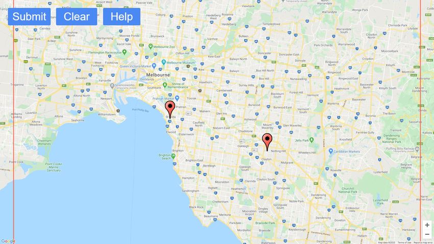
system are presented in Section 3. The details of our user
Manchester implemented both of these techniques, as well as the full routing algorithm, and can
Manchester
demonstrate choice routing running over any combination.
study and its results are presented in Section 4. Some lim- Whichever way the trees are computed, so long as they cover sufficient roads to
Cambridge Cambridge
identify the optimum route, they must also be exploring the other near-optimal routes
itations of the user study are also discussed in Section 4. to some extent, and our method of combining the trees will yield the good choices.
1.2.6 Enumerating the Plateaux
Section 5 concludes this paper. Once the links that are parts of plateaux are marked, we scan all of the links,
following plateaux as we find them, marking the links as traversed, and keeping a
note of the length of the plateau and the link that generated it. We keep a note of the
longest n plateaux found in this way. When the scan has finished, we have a list of the
longest n plateaux that have been generated by combining the trees.
2. RELATED WORK We can generate a full route from a plateau by choosing any point in the plateau, and
tracing it back to A in the source tree, and to B in the destination tree.
There will be many such routes, some generated by only tiny plateau. What we look
for are the longest plateau. Actually, where we refer to “longest”, we really mean
Computing alternative routes has received significant re- “highest cost”. We also want routes that are not too much longer than the single most
optimal route. The simplest assessment is to use the length of the chain, minus the
length of the overall generated route. Call this C - R. This can be expressed as the
search in the past decade or so [11, 2, 7, 3, 10, 9, 12]. In this Figure 1. Source tree from Cambridge
amount of the generated route that is outside of the chain, and can be simply
computed from valuesFigure
stored2.in Destination
the trees. It istree
a negative quantity, and the less
to Manchester
section, we briefly describe some of the most popular tech- (a) Tf rooted at Cambridge (b) Tb rooted at Manchester
Another by-product of the computation of this tree is that for each point, we have
computed and stored the cost of the minimum cost route from the origin A to that
negative it is, the better the route.
This quantity can be used to rank the routes in order of preference, and we find that
the routes that we are interested in are indeed brought to the fore.
point. 1.2.3 Plateaux in Combined Cost
niques and focus on presenting the details of the three tech- 1.2.2 Destination Tree
We now look for sequences of directly linked points that are found in both trees, in
the same order. These are chains that are both good for getting away from A and
niques that we compare in this user study: Penalty, Plateaus We then compute the single most optimum routes from all nodes to the destination B.
Manchester
These are a tree that contains chains of points that form the good routes for getting Manchester 5
towards B. Any good route from A to B is going to involve some of these chains. The
longer the chains are, the better they are going to be in getting from A to B.
and Dissimilarity.
towards B.
1
The chains represent the best roads in their area that are well-aligned for getting from
Cambridge A to B, which is just what we are after.
Cambridge
To find these chains, we begin by adding together the costs from each tree. For a
3
general point C, the source tree gives us the cost of follwing the optimum route from
A to C. The cost from the destination tree gives us the cost of following the optimum
2.1 Penalty 4
route from C to B. Thus the sum of these costs at C gives us the cost of the optimum
route from A to B via C.
2
If there is a point D that adjoins C and where a link from C to D is contained in both
The basic idea behind this technique [3, 7] is to iteratively trees, then the cost in one tree will increase by exactly the amount by which it
decreases in the other tree, so the sum remains the same. Thus the chains that we are
interested in are characterised in that the cost-sum at each node in the chain is
compute shortest paths and, after each iteration, apply a constant. The route involving the chain will begin at the source node where the cost-
sum is the cost of the optimum route from A to B. As the route proceeds towards C, if
C is not on the optimal route, that cost-sum will rise at some nodes, then reach and
penalty on each edge of the shortest path found in the pre- stay at the cost-sum at C for some while (the length of the chain), then decrease at
some nodes until the destination is reached. For this reason, we call the chain a
plateau. We find these by grouping together all sets of nodes that have the same cost-
vious iteration (by increasing its weight by a certain factor). sum and that are connected directly by a link.
Figure 3. Combination tree Figure 4. Plateau routes
Since the edge weights of the previous shortest paths are (c) Tree Join
1.2.4 Plateaux by Back Pointers
(d) Plateau-based paths
Another way to find the links that are in the plateaux is to mark links that have back
increased, it is likely that the new shortest path found on pointers in the source tree pointing to them, and the links that have back pointers in
the destination tree pointing to them. Then, if a link has both marks, it is part of a
the graph will be different from the previous path(s). The Figure 1: Alternative paths using plateaus. Images
plateau. It is essential to use the back pointers rather than the costs if the trees have
been computed using a time-dependent cost function.
algorithm stops when k shortest paths are retrieved. adapted from [11] with permission.
1.2.5 Compatibility with routing optimisations
Many routing engines compute only a subset of the source or destination tree.
This approach does not guarantee that the paths are “sign- One approach is to preferentially search roads in the direction of the destination, using
a variant of the A* algorithm. In this case, the trees will explore roughly elliptical
areas with A and B as the foci of the ellipse. These trees must still cover all feasible
ficiantly” different from each other or are meaningful (e.g., routes (otherwise they might miss the optimum), and so when they are combined, they
still yield the same choice routes.
without small detours). However, we observe that, in prac- consists of generating two shortest path trees (e.g., using Di-
Another approach is to route along a subset of roads which are known to be better for
use in crossing the country, which we will call priority roads. Of course, local roads
must be searched in the vicinity of the source and destination, but the main
tice, the routes generated by this approach turn out to be jkstra’s algorithm) and joining the two trees. The latter can
computation across the space between source and destination is vastly reduced by
only searching along this subset of known good roads. Again, the trees must cover
most feasible routes, otherwise the optimum could be missed. The trees can therefore
pretty good in most of the cases. This is mainly because, be done in time linear to the size of the tree [11]. Thus, the
be combined in the usual way to identify the plateau, and a set of choice routes is
generated.
For the ultimate in computation speed and memory reduction, the techniques above
on typical road networks, there exists several different paths total cost is dominated by the two Dijkstra searches.
can be combined, and other clever optimisations may also be used. We have
from s to t with very similar traveling time. Thus, when
the algorithm applies penalty to one of these paths, it nat- 2.3 Dissimilarity
urally tends to select the other significantly different paths. Some existing works [10, 9, 12] specifically define a dis-
Furthermore, after retrieving each path, the algorithm can similarity function dis(p, P ) to compute the dissimilarity of
specifically apply additional filtering criteria to remove the a candidate path p to a set of paths P . The aim is to iter-
paths that fail to meet certain requirements, e.g., the paths atively add paths to the result set P in ascending order of
that are too similar to existing paths or have detours. their lengths as long as they are sufficiently dissimilar to the
previously selected paths. Specifically, a path p is added to
2.2 Plateaus P only if dis(p, P ) > θ where θ is a user-defined dissimilarity
The technique to generate alternative paths using plateaus threshold. As a result, the k paths reported to the user are
was developed [11] by Cotares Limited for their routing en- significantly different to each other and are short.
gine Choice Routing. We use Fig. 1 to illustrate how al- The advantage of this approach is that it guarantees that
ternative paths from Cambridge (source s) to Manchester the alternative paths are sufficiently dissimilar to each other
(target t) are generated using plateaus. First, two shortest (as defined by the parameter θ). However, this approach
path trees are generated: a forward shortest path tree Tf does not guarantee that the generated alternative paths are
rooted at s (see Fig. 1(a)); and a backward shortest path free of small unnecessary detours. This can be addressed by
tree Tb rooted at t (Fig. 1(b)). Then, the two trees Tf and having additional filtering criteria to prune the paths that
Tb are joined to obtain the branches common in both trees. do not meet certain criteria. A major disadvantage of this
These common branches are called plateaus. Fig. 1(c) shows approach is that the problem is NP-hard [10, 12]. The exist-
some of the most prominent plateaus. It was noted [11] that ing studies have proposed several approximate algorithms.
longer plateaus result in more meaningful alternative paths. However, many of these techniques still appear to be too
Therefore, top-k plateaus are selected based on their lengths. slow taking tens of seconds to report alternative paths on a
Let u and v be two ends of a plateau pl(u, v) where u is the city-scale road network.
end closer to the source and v is the end closer to the target. In this study, we use SSVP-D+ [9] which has been shown
Each plateau pl(u, v) is used to generate an alternative path to generate good quality alternative routes and has reason-
by appending the shortest paths from s to u and v to t to able computation time. The basic idea is to use via-nodes to
the plateau. Fig. 1(d) shows five alternative paths generated generate paths. A path (called via-path) generated using a
using the five longest plateaus from Fig. 1(c). via-node u is the concatenation of sp(s, u) and sp(u, t) where
It was shown that the alternative paths generated using sp(x, y) denotes the shortest path from x to y. To efficiently
plateaus are local optimal [2]. Furthermore, the plateaus compute sp(s, u) and sp(u, t), similar to the plateaus-based
do not intersect each other. Thus, two paths generated us- approach, two shortest path trees are constructed rooted at
ing longer plateaus are expected to have a smaller overlap s and t, respectively. The algorithm iteratively selects via-
(i.e., lower similarity). Thus, the paths generated using the nodes in an ascending order of their via-paths lengths. A
k longest plateaus are likely to be more dissimilar to each via-path is added to the result set only if its dissimilarity to
other. The computational cost to compute alternative paths the existing paths in P is greater than the threshold θ.
2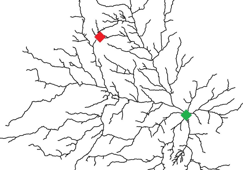
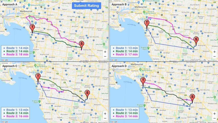
(a) A user selects source and target locations                 (b) Alternative routes by each approach are displayed

                                                  Figure 2: User Interface

                                                                     user-interface; 3) query processor. We briefly describe each
                                                                     component below.
                                                                     Road Network Constructor: The road network construc-
                                                                     tor takes a rectangular area as input and extracts the road
                                                                     network data from OpenStreetMap (OSM) that lies within
                                                                     the input rectangle. We design our demo system to allow
                                                                     routing queries only in Melbourne Metropolitan area, i.e.,
                                                                     the input rectangle covers the Melbourne Metropolitan area.
                                                                     First, we export the raw OSM data using Geofabrik3 . Then,
                                                                     we filter the data that lies in the input rectangle. Finally,
                                                                     we parse the content of this raw OSM data to generate the
                                                                     road network data needed for the approaches. Specifically,
                                                                     we extract tuples where each tuple represents an edge of the
                                                                     road network along with its end vertices and edge weight
                                                                     (travel time). The travel time is obtained by dividing the
                                                                     length of the edge with the maximum speed along the edge.
                                                                     In real-world scenarios, the vehicles may need to stop at in-
                                                                     tersections, wait at traffic lights or slow down while turning
                Figure 3: Feedback form                              even when there is no congestion on the roads. Thus, esti-
                                                                     mating the travel time using maximum speed is not realistic.
                                                                     To better simulate real-world scenarios, for each road seg-
2.4     Other techniques                                             ment that is not a freeway/motorway, we multiply the edge
   Yen’s algorithm [14] can be used to compute k shortest            weight (travel time) by 1.3. Our trials showed that this
paths from s to t. However, these k shortest paths are all           results in a reasonably good estimate of actual travel time
expected to be very similar to each other. Thus, Yen’s al-           when the roads have no congestion (e.g., compared with the
gorithm is not suitable for generating alternative paths if          travel time estimated by Google Maps at 3:00 am).
applied trivially. However, some existing techniques (e.g.,          User Interface: The user interface is a dynamic web page
see [8]) use Yen’s algorithm to incrementally generate short-        created using HTML, Javascript, and JQuery. It has two
est paths and apply filtering techniques to prune the paths          main functionalities: (1) sending the user’s query request to
that do not meet certain criteria. Pareto optimal [5, 6] paths       the back-end, and (2) interacting with Google Maps API 4
(i.e., skyline paths) report the paths that are not dominated        to plot the routes on Google Maps. More specifically, ini-
by any other path according to given criteria (e.g., distance,       tially, it displays Melbourne region on Google Maps. A user
travel time and ease of traveling). Many techniques use              can click anywhere on the map within a specified rectangular
via-nodes to generate alternative paths (e.g., the SSVP-D+           area (corresponding to the Melbourne Metropolitan area) to
techniques discussed in Section 2.3). Such techniques iden-          pick two markers corresponding to the source and target lo-
tify interesting via-nodes in the road network and then ap-          cations, respectively (see Fig. 2(a)). When the user presses
ply different filtering/ranking criteria to generate the top-k       the “Submit” button, the source and target locations are
alternative paths.                                                   sent to the back-end which computes the alternative routes
                                                                     generated by the Penalty, Plateaus and Dissimilarity tech-
                                                                     niques. Additionally, the routes generated by Google Maps
3.     DEMONSTRATION SYSTEM                                          are also obtained by calling its API. The routes generated
  Our web-based demonstration system2 consists of the fol-           by each of the four approaches are then displayed in a new
lowing major components: 1) road network constructor; 2)             3
                                                                         http://download.geofabrik.de/
2                                                                    4
    http://aamircheema.com/routing/demo.html                             https://developers.google.com/maps/documentation/

                                                                 3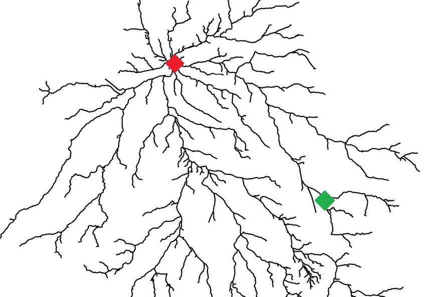
window (see Fig. 2(b)). The approaches are named A-D (A:             4.1    Results
Google Maps, B: Plateaus, C: Dissimilarity and D: Penalty).             We show the results (mean rating and standard devia-
This is to hide the identities of the approaches from the            tion) for each approach for different groups of participants
users, to avoid any biases or preconceived notions.                  (Melbourne residents vs non-residents). We also group the
   The user can rate each approach by clicking on the “Sub-          responses based on the lengths of the shortest routes from
mit Rating” button which opens a form as shown in Fig. 3.            source to target locations. Specifically, small routes corre-
Specifically, the form requires the user to rate each approach       spond to all the responses where the fastest travel time from
from 1-5 (higher is better). We also ask the users whether           s to t was at most 10 minutes. Medium and long routes cor-
they are currently living (or have lived) in Melbourne. This         respond to the responses with fastest travel time from s to
enable us to analyse the results based on the ratings received       t within ranges (10, 25] and (25, 80] minutes, respectively.
by Melbourne residents vs non-residents.                             The highest mean rating for for each group is shown using
Query Processor: The input to the query processor is a               bold font.
pair of source and target locations each represented by longi-          The results in Table 1 show the results for all respon-
tude and latitude. First, the query processor performs geo-          dents. The Plateaus achieves the highest mean rating and
coordinate matching and selects the closest vertices from            Google Maps the lowest considering all responses. It is also
the OSM data to the source and target locations, respec-             interesting to note that Penalty has the highest mean rating
tively. Then, the query processor computes the alternative           for the small routes whereas Dissimilarity and Plateaus per-
routes from the source location to the target location using         form better for the medium and long routes, respectively.
the three techniques we implemented (Penalty, Plateaus and           Also note that the difference between the mean ratings of
Dissimilarity). It also calls Google Maps API to get the al-         Google Maps and the other approaches shrinks, considering
ternative routes generated by Google Maps. For each of the           responses only from Melbourne residents. This indicates
routes generated by these four approaches, the query proces-         that the routes provided by Google Maps may be perceived
sor computes its travel time by using the OSM data. Each             to be of poor quality by non-residents when in fact they may
travel time is rounded to display time in minutes. Finally,          not be necessarily so. Next, we provide detailed results con-
the routes generated by each approach are passed to Google           sidering responses only from Melbourne residents (Table 2)
Maps API to display these routes using different colors so           and non-residents (Table 3).
that they are easily distinguishable.                                   Table 2 shows the results considering responses only from
Parameter Details: The three approaches that we imple-               the Melbourne residents. Dissimilarity achieves the high-
mented (Penalty, Plateaus and Dissimilarity) use some pa-            est overall mean rating whereas Plateaus and Penalty have
rameters. As suggested in [4], for the Penalty approach,             marginally lower mean ratings. As earlier, Penalty per-
the penalty that we apply to each edge is 1.4, i.e., the edge        forms the best for the small routes whereas Dissimilarity
weight is multiplied by 1.4. For the Plateaus and Dissimilar-        and Plateaus have the highest mean ratings for medium and
ity approaches, we use the upper bound [2] to be 1.4 which           long routes, respectively. The results considering only the
ensures that the travel time of any alternative path reported        non-residents are shown in Table 3. Plateaus achieves the
by these approaches is not higher than 1.4 times the travel          highest mean rating whereas the Google Maps the lowest.
time of the fastest path. The dissimilarity threshold θ for          Interestingly, the mean rating for each approach is smaller
the Dissimilarity approach is set to 0.5 as suggested by the         compared to the mean rating received by Melbourne resi-
relevant studies [9, 10]. We tried several other values for          dents (significantly smaller for medium routes).
each of the above mentioned parameters to confirm that the              We also conducted one-way ANOVA tests for different
chosen values are appropriate.                                       categories of respondents. Given a null hypothesis of no
                                                                     statistically significant difference in mean ratings of the four
4.     USER STUDY                                                    approaches, the p-value is relatively high (p-value=0.16 con-
                                                                     sidering all respondents, p-value=0.68 for Melbourne resi-
  We created a webpage5 explaining the purpose and back-
                                                                     dents and p-value=0.18 for non-residents) suggesting that
ground of this research and providing instructions to the
                                                                     there is no evidence that the null hypothesis is false, i.e.,
participants. The participants were able to provide feed-
                                                                     there is no credible evidence that the four approaches re-
back using any internet enabled device (e.g., laptop, tablets
                                                                     ceive different ratings on average.
or smartphones). We sent the requests for participation in
the study via emails and personal messages. Most of the
requests were sent to the people living in Melbourne who
                                                                     4.2    Limitations of the study
were likely to be familiar with the roads. For the sake of              While we have tried our best to be as fair as possible to
this study, we say a participant is Melbourne resident if            all the approaches, certain factors may have affected the
he/she was living (or had lived) in Melbourne at the time            participants’ perceived quality of the routes. Below we list
of participation. We also sent requests to non-residents to          some of these.
get their ratings for each approach based on their perceived         Different data used by Google Maps and other ap-
route quality. The Melbourne residents were requested to             proaches: One of the major factors (beyond our control)
select the source and target locations for the routes familiar       potentially affecting the participants’ ratings is that the data
to them (although we cannot guarantee if they always did             used by Google Maps and the OpenStreetMap (OSM) data
so). We made sure that none of the approaches tries to avoid         used by the other three approaches are different. To estimate
toll roads and we told the participants to ignore toll charges       the travel time, Google Maps uses real-time traffic data (or
on the roads. In total, we received 237 responses (156 from          historical data for queries issued at future dates/times). To
Melbourne residents and 81 from non-residents).                      minimize the impact of real-time traffic or historical traf-
                                                                     fic data, we call Google Maps API to retrieve the routes
5
    http://aamircheema.com/routing                                   at 3:00 am on the next day (assuming minimal traffic on

                                                                 4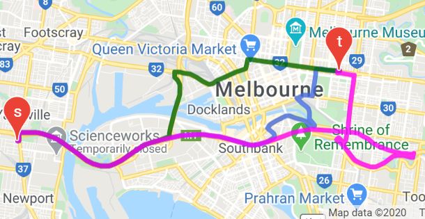
Google Maps          Plateaus     Dissimilarity       Penalty       #Responses
    Overall                                 3.37 (1.33)        3.63 (1.25)    3.58 (1.29)       3.56 (1.17)       237
    Melbourne residents                     3.55 (1.28)        3.69 (1.17)    3.70 (1.22)       3.66 (1.12)       156
    Non-residents                           3.04 (1.37)        3.51 (1.38)    3.34 (1.37)       3.37 (1.25)        81
    Small Routes (0, 10] (mins)             3.53 (1.17)        3.48 (1.27)    3.69 (1.18)       3.81 (1.08)        66
    Medium Routes (10, 25] (mins)           3.44 (1.39)        3.51 (1.27)    3.58 (1.26)       3.42 (1.23)       109
    Long Routes (25, 80] (mins)             3.11 (1.36)        3.98 (1.13)    3.45 (1.44)       3.54 (1.14)        62

    Table 1: All responses: Mean rating m and standard deviation sd for each approach shown as m(sd).

                                           Google Maps          Plateaus     Dissimilarity       Penalty       #Responses
    Melbourne residents                     3.55 (1.28)        3.69 (1.17)    3.70 (1.22)       3.66 (1.12)       156
    Small Routes (0, 10] (mins)             3.50 (1.16)        3.42 (1.27)    3.68 (1.25)       3.97 (0.99)        38
    Medium Routes (10, 25] (mins)           3.64 (1.28)        3.70 (1.14)    3.78 (1.13)       3.55 (1.17)        83
    Long Routes (25, 80] (mins)             3.40 (1.42)        3.97 (1.10)    3.54 (1.44)       3.60 (1.09)        35

         Table 2: Only Melbourne residents: Mean rating and standard deviation for each approach

                                           Google Maps          Plateaus     Dissimilarity       Penalty       #Responses
    Non-residents                           3.04 (1.37)        3.51 (1.38)    3.34 (1.37)       3.37 (1.25)       81
    Small Routes (0, 10] (mins)             3.57 (1.20)        3.57 (1.29)    3.71 (1.08)       3.61 (1.17)       28
    Medium Routes (10, 25] (mins)           2.81 (1.55)        2.92 (1.47)    2.96 (1.48)       3.00 (1.33)       26
    Long Routes (25, 80] (mins)             2.74 (1.23)        4.00 (1.21)    3.33 (1.47)       3.48 (1.22)       27

             Table 3: Only non-residents: Mean rating and standard deviation for each approach

                   (a) Routes by Google Maps                                      (b) Routes by Plateaus

Figure 4: Blue and Green routes by both approaches are the same. The purple route by Google Maps looks
more complicated and has higher travel time than the purple route by Plateaus when OpenStreetMap data
is used but has smaller travel time when Google Maps data is used to compute the travel time.

roads at that time). However, the travel time estimation for       taken by Plateaus is a few minutes higher than that of the
the same route may still be different for Google Maps and          purple route by Google Maps. A user looking at the routes
OpenStreetMap data. We observe that this difference in             in Fig. 4 is likely to give a higher rating to Plateaus but this
the underlying data affects the routes generated by Google         may be unfair because the two approaches are essentially
Maps and the other approaches.                                     using different underlying data.
   Consider the example given in Fig. 4 that shows the al-         Apparent detours that are not: Due to the complex
ternative routes generated by Google Maps and Plateaus             structure of road networks, a participant may incorrectly
for the same pair of source and target. While the blue and         assume that a route provided by an approach has a detour.
green routes returned by both approaches are the same, the         In the example of Fig. 4(a), the purple route by Google
purple route returned by Google Maps looks significantly           Maps appears to have a detour, e.g., one may assume that
more complicated and appears to have detours. We care-             the route should have turned left at around “Shrine of Re-
fully looked into the purple routes provided by the two ap-        membrance” instead of the detour. However, this is not a
proaches. It turns out that if the data from OpenStreetMap         detour because the route goes through a tunnel and there
is used, the travel time of the purple route by Google Maps        is no left turn available near “Shrine of Remembrance”, i.e.,
is a few minutes higher than that of the purple route by           the path returned by Google Maps is a reasonable path. Un-
Plateaus. However, when Google Maps data is used to ob-            less a user is familiar with these roads and/or carefully looks
tain the travel times (by forcing Google Maps to generate a        at the road structure (e.g., by zooming in), he/she may per-
path taken by Plateaus), the travel time of the purple route       ceive it as a detour and give a lower rating. We remark

                                                               5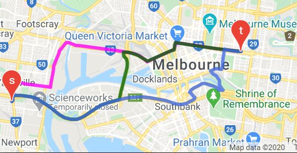
that this does not only negatively affect the ratings received         that of Google Maps, one-way ANOVA test shows that the
by Google Maps. Other approaches may also be negatively                results are not statistically significant. We also identify the
affected by such scenarios where a user may incorrectly as-            limitations of this study that might have potentially affected
sume a reasonable route to have detours.                               the ratings submitted by the participants. Despite the limi-
Biases to favorite routes/navigation systems: A par-                   tations of the study, we believe that it is fair to conclude that
ticipant’s rating may be biased by his/her favorite routes (or         the three approaches (Plateaus, Dissimilarity and Penalty)
his/her favorite navigation system). E.g., a person who reg-           are promising and the quality of routes generated by them is
ularly uses Waze to travel from home to office may perceive            at least comparable to the routes provided by Google Maps.
the routes that are similar to those provided by Waze to
have a better quality, although this may not be necessarily            6.   REFERENCES
true. For example, one participant submitted the following
                                                                        [1] I. Abraham, D. Delling, A. V. Goldberg, and R. F.
comment: “no route using Blackburn rd”. We believe that
                                                                            Werneck. A hub-based labeling algorithm for shortest
the route via Blackburn road is his/her favorite route which
                                                                            paths in road networks. In International Symposium
was not returned by any of the approaches. Consequently,
                                                                            on Experimental Algorithms. Springer, 2011.
the maximum rating the user gave to any approach in this
case was 3.                                                             [2] I. Abraham, D. Delling, A. V. Goldberg, and R. F.
Additional filtering/ranking criteria are not consid-                       Werneck. Alternative routes in road networks. Journal
ered: For the approaches that we implemented (Plateaus,                     of Experimental Algorithmics (JEA), 18:1–3, 2013.
Dissimilarity and Penalty), we could choose to use some                 [3] V. Akgün, E. Erkut, and R. Batta. On finding
additional filtering/ranking criteria to refine the top-k al-               dissimilar paths. European Journal of Operational
ternative routes. For example, we could improve the routes                  Research, 121(2):232–246, 2000.
generated by Penalty and Plateaus by pruning the alterna-               [4] R. Bader, J. Dees, R. Geisberger, and P. Sanders.
tive routes that have very high similarity to the other routes.             Alternative route graphs in road networks. In
Similarly, we could filter the routes in Penalty and Dissim-                International Conference on Theory and Practice of
ilarity approaches that did not satisfy local optimality [2].               Algorithms in (Computer) Systems, 2011.
Some comments from the participants also point out that,                [5] F. Barth and S. Funke. Alternative routes for next
at least some, users consider certain factors to be important               generation traffic shaping. In Proceedings of the 12th
which we did not consider in our implementation but can be                  ACM SIGSPATIAL International Workshop on
easily included.                                                            Computational Transportation Science, 2019.
   For example, some comments from the participants were:               [6] F. Barth, S. Funke, and S. Storandt. Alternative
“Approach C provides paths with less turns”; “less zig-zag                  multicriteria routes. In Proceedings of the
is better”; and “highest rated path follows wide roads”. This               Twenty-First Workshop on Algorithm Engineering and
indicates that these users perceive the routes to be better if              Experiments, ALENEX 2019, San Diego, CA, USA,
they have fewer turns or are using wider roads (which prob-                 January 7-8, 2019, pages 66–80, 2019.
ably means roads with more lanes). Since Google Maps is a               [7] Y. Chen, M. G. Bell, and K. Bogenberger. Reliable
widely used commercial product, we believe that they would                  pretrip multipath planning and dynamic adaptation
have spent significant time and resources to identify such po-              for a centralized road navigation system. IEEE
tentially important factors and implement additional filter-                Transactions on Intelligent Transportation Systems,
ing/ranking criteria to report alternative routes. However,                 2007.
most of these filtering criteria can also be easily included for        [8] T. Chondrogiannis, P. Bouros, J. Gamper, and
the other approaches but are not considered in this study.                  U. Leser. Alternative routing: k-shortest paths with
   Considering the factors mentioned above (and the other                   limited overlap. In SIGSPATIAL, 2015.
unforeseen factors), we recommend the readers to make any               [9] T. Chondrogiannis, P. Bouros, J. Gamper, U. Leser,
conclusions with caution. However, we believe that our                      and D. B. Blumenthal. Finding k-dissimilar paths with
study shows evidence that the three approaches that we im-                  minimum collective length. In SIGSPATIAL, 2018.
plemented (Plateaus, Dissimilarity and Penalty) are at least           [10] T. Chondrogiannis, P. Bouros, J. Gamper, U. Leser,
comparable to Google Maps. We also received some com-                       and D. B. Blumenthal. Finding k-shortest paths with
ments from the participants indicating that they find the                   limited overlap. The VLDB Journal, pages 1–25, 2020.
routes to be of similar quality. For example a participant
                                                                       [11] A. H. Jones. Method of and apparatus for generating
commented: “I don’t see these approaches as very distinct
                                                                            routes, Aug. 21 2012. US Patent 8,249,810.
from each other.”. Another participant sent a personal mes-
sage to the authors stating that he is finding it hard to rank         [12] H. Liu, C. Jin, B. Yang, and A. Zhou. Finding top-k
the approaches since they all seem to be of similar quality.                shortest paths with diversity. IEEE Transactions on
                                                                            Knowledge and Data Engineering, 2017.
                                                                       [13] D. Ouyang, L. Yuan, L. Qin, L. Chang, Y. Zhang, and
5.   CONCLUSIONS                                                            X. Lin. Efficient shortest path index maintenance on
  This is the first detailed user study that compares some of               dynamic road networks with theoretical guarantees.
the most popular approaches to generate alternative routes,                 Proceedings of the VLDB Endowment, 2020.
including Google Maps which is one of the most widely used             [14] J. Y. Yen. Finding the k shortest loopless paths in a
navigation applications. We develop a web-based demo sys-                   network. management Science, 17(11):712–716, 1971.
tem to conduct the user study. Our results show that the
three approaches published in the literature provide alter-
native routes of similar quality to each other. Although the
mean ratings received by these approaches is higher than

                                                                   6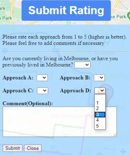
You can also read


