GeoGAN: A Conditional GAN with Reconstruction and Style Loss to Generate Standard Layer of Maps from Satellite Images
←
→
Page content transcription
If your browser does not render page correctly, please read the page content below
GeoGAN: A Conditional GAN with Reconstruction
                                             and Style Loss to Generate Standard Layer of Maps
                                                            from Satellite Images

                                                                      Swetava Ganguli∗, Pedro Garzon, Noa Glaser
arXiv:1902.05611v2 [cs.CV] 25 Apr 2019

                                                                           Department of Computer Science
                                                                        Stanford University, Stanford, CA 94305
                                                                    {swetava,pgarzon,nglasr}@cs.stanford.edu

                                                                                          Abstract

                                                     Automatically generating maps from satellite images is an important task. There
                                                     is a body of literature which tries to address this challenge. We created a more
                                                     expansive survey of the task by experimenting with different models and adding
                                                     new loss functions to improve results. We created a database of pairs of satellite
                                                     images and the corresponding map of the area. Our model translates the satellite
                                                     image to the corresponding standard layer map image using three main model
                                                     architectures: (i) a conditional Generative Adversarial Network (GAN) which
                                                     compresses the images down to a learned embedding, (ii) a generator which is
                                                     trained as a normalizing flow (RealNVP) model, and (iii) a conditional GAN where
                                                     the generator translates via a series of convolutions to the standard layer of a map
                                                     and the discriminator input is the concatenation of the real/generated map and the
                                                     satellite image. Model (iii) was by far the most promising of three models. To
                                                     improve the results we also added a reconstruction loss and style transfer loss in
                                                     addition to the GAN losses. The third model architecture produced the best quality
                                                     of sampled images. In contrast to the other generative model where evaluation of
                                                     the model is a challenging problem. since we have access to the real map for a
                                                     given satellite image, we are able to assign a quantitative metric to the quality of the
                                                     generated images in addition to inspecting them visually. While we are continuing
                                                     to work on increasing the accuracy of the model, one challenge has been the coarse
                                                     resolution of the data which upper-bounds the quality of the results of our model.
                                                     Nevertheless, as will be seen in the results, the generated map is more accurate
                                                     in the features it produces since the generator architecture demands a pixel-wise
                                                     image translation/pixel-wise coloring. A video presentation summarizing this paper
                                                     is available at: https://youtu.be/Ur0flOX-Ji0

                                         1       Introduction
                                         Creating maps is a very expensive and time consuming process; yet it is one of the most important
                                         sources of curated data. Maps have commercial value to companies in multiple sectors of the
                                         economy: ride-sharing companies (like Uber and Lyft), food delivery companies like (like DoorDash
                                         and GrubHub), national security agencies (like CIA, NSA, and FBI), and many other sectors of the
                                         economy. It is important to emphasize that in addition to the map being accurate, most of the apps
                                         created by the companies mentioned above have a major human-interaction component associated
                                         with their success. For e.g. Customers interact with a map interface while tracking their ride on the
                                         Uber/Lyft app while apps that geo-code photographs taken on a device present the pictures associated
                                             ∗
                                                 Corresponding Author

                                         Preprint. Work in progress.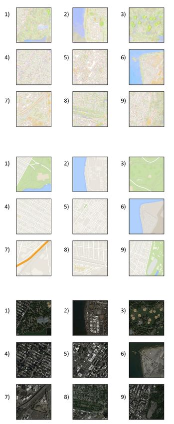
with a given geographic location on a human-readable map interface. Constructing accurate maps
has been a major push for companies that want to sell “smart devices” since a major part of what
makes a device smart is its ability to locate itself and inform its user via a human-readable interface.
More importantly, maps have a huge humanitarian value. For e.g., generating an accurate map of
refugee camps can aid the timely delivery of food and resources to the people in these camps. A map
may be also viewed as data that is not necessarily machine readable. This approach is suitable in the
domain of autonomous vehicles and self-driving cars. An accurate map must reflect all changes on the
ground in a timely manner. Up-to-date geospatial data is continuously collected from flyover imaging
air-crafts or satellites. Currently, there is considerable latency between changes to geographic/road
conditions on the ground and the publicly available human-readable maps. One way to reduce this
latency is to automate the process of human-readable map generation from a satellite image of a
given location at a specified zoom level and resolution. In this work, we emphasize the importance
of human-readability of a map and aim to construct accurate human-readable maps directly from a
satellite/aerial image of the location. The satellite/aerial image specifies the zoom level and resolution
of the required map. The style of the generated human-readable map is chosen to be the style of
the publicly available Google Maps API. Satellite images are obtained from the publicly available
Google Earth Engine datasets and its corresponding map is obtained using the Google Maps API.
The process of querying these databases and aligning the satellite/aerial image with its corresponding
map is described in the section on datasets.

2   Related work

Image-to-Image translation has been a recent development and area of research in the field of
generative modeling. One of the most recent successes is the work of Chan et al. (2018). The use of
GANs (Goodfellow et al. (2014)) for novel generative tasks has exploded over the past few years
due to better training algorithms (Gulrajani et al. (2017)) and novel ways to define the loss function
which must be optimized (Arjovsky, Chintala, and Bottou (2017)). Costea et al. (2017) proposed the
dual-hop GAN (DH-GAN) to detect roads and intersections and used that to find its best covering road
graph by applying a smoothing-based graph optimization procedure. In addition, using convolutional
neural networks and GANs on geospatial data in unsupervised or semi-supervised settings has also
been of interest recently; especially in domains such as food security, cybersecurity, satellite tasking,
etc. (Ganguli, Dunnmon, and Hau (2019); Perez et al. (2019); Dunnmon et al. (2019)). Conditional
Adversarial Networks (Mirza and Osindero (2014); Isola et al. (2016)) have been used to perform
general purpose image-to-image translation. The recently proposed CycleGAN architecture has been
evaluated on satellite imagery to map translation (Zhu et al. (2018)). GANs have been also used
to create spoof satellite images and spoof images of the ground truth conditioned on the satellite
image of the location (Xu and Zhao (2018)). Conditional GANs have also been used to generate
ground-level views of locations from overhead satellite images Deng, Zhu, and Newsam (2018).
As an alternative to standard neural network generators, there has also been progress and recent
models proposed based on normalizing flow models that use invertible bijections of distributions
to convert one distribution to another and back again. An alternative architecture for the generator
in a GAN would be a normalizing flow model which takes advantage of the bijective mapping
between the input noise/condition vector and the generated image and could in principle be used
to gain more insight by training the model to seek disentangled latent representations of the map.
Recently proposed normalizing flow models that have succeeded in face generation is the Real-Valued
Non-Volume Preserving Normalizing Flow Model (RealNVP). The RealNVP has been shown to
have decent success in the task of photorealistic face generation (Dinh, Sohl-Dickstein, and Bengio
(2016)) and disentangling its latent representations. In this project, we modify the conditional GAN
architecture in various ways to obtain the one best suited for our task of generating a map for a location
given the satellite/aerial image of the location. In addition to experimenting with new architectures,
we also analyze the importance of different flavors of loss functions that penalize the model on certain
specified quantitative metrics of generated sample quality to get a more comprehensive survey of
the task. We also contribute code that provides a scalable method to generate new datasets from the
publicly available Google Earth Engine and the Google Maps APIs.

                                                    2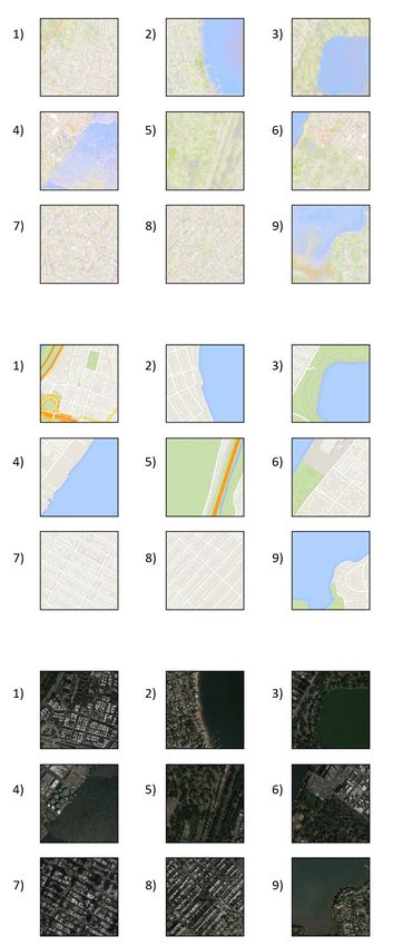
3     Task Definition
GeoGAN is a model that takes as its input a satellite image at a specified zoom level and resolution
and produces the corresponding human-readable map for that location. The model is trained to
emulate the style of the maps available from the Google Maps API for the generated map. The
emphasis in this paper is on the accuracy of the generated map. As opposed to many generative
tasks, we have access to the real map corresponding to a satellite image which is obtained from the
Google Maps API. The model is trained as a conditional GAN with the input satellite image as the
condition for the generation of the map. While it is relatively straightforward to condition the output
of a generator, there is no clear way to condition the output of the discriminator. We perform several
experiments on the methods to condition the discriminator. For most of our experiments, our inputs
are 64x64x3 (3 channel) satellite images which are translated into 64x64x3 map images. However,
for the model christened “model 3”, we use 256x256x3 dimensional satellite images to generate
256x256x3 maps.

3.1   Datasets

We need tiles with corresponding spatial resolution at locations at specific (latitude, longitude) pairs
from street maps, overhead imagery, and geospatial elevation datasets. We built pipelines to download
the images from Google Earth engine and the Google Maps API. Our pipeline first calculates a
set of lat/long coordinates to span a given city. These lists of coordinates are then fed into scripts
downloading data from Google Earth Engine and Google Maps. Then, a third script matches the
images and stores them as Tensorflow data records containing corresponding satellite images and
map tiles. So far we have extracted images from San Francisco, Seattle, New York, Austin, Miami,
Washington D.C., Boston, and Chicago for a total of 41756 for both training and test, of which we
cleaned out 7605. For satellite imagery, we will be using Sentinel2 from Google Earth Engine, which
has a 10m pixel resolution over the red/green/blue NIR bands Engine (2018). A benefit of using this
data source for satellite images is that querying is free and you also get access to other channels such
as an infrared red channel. It also contains other views that better topographic representation of a
location. Because the ground looks different in different parts of the year, we download images from
around March, June, September, and December from each region. We used the provided cloud-mask
channel to select the images with the least clouds. If no images in a month contain less than 10%
cloud coverage, we extend the dates region. For satellite imagery, we also have access to higher
resolution digital globe data from the DeepGlobe challenges. However we are not using this data at
the moment. The roads challenge dataset, for example, consists of 6226 satellite images of 1024 x
1024 pixels with a 50cm pixel resolution in the RGB bands Demir et al. (2018). This fine resolution
is great and future work might explore incorporating this data. For the maps data, we will be using
tiles from the Google Maps Static API. This API allows us to retrieve tiles from anywhere in the
globe without street labels and at a few specific discrete zoom levels. We have opted to use zoom
level 14, which roughly translates to 7.242090 meters per pixel resolution as 512 x 512 PNG images.
We form our tiles by going to the top left corner of a city all the way to the bottom right corner. In
addition to our handcrafted dataset, we also compare using the collected dataset from UC Berkeley
researcher Taesung Park that uses the Google Maps API to scrape both satellite and map images of
size 256 x 256 from New York City Park (2018).

4     Technical Approach
4.1   Our Contributions

Zhu et al. (2018) present the CycleGAN architecture which translates satellite imagery to maps. In
this paper, we experiment with and propose alternate novel architectures and loss functions to train
for this task.

       1. A Conditional GAN emulating the architecture proposed by Mirza and Osindero (2014)
          where the satellite images are first passed through an encoder to compress them to a lower
          dimensional vector. We experiment with both, an approach where the encoder is trained
          end-to-end, and an approach where the encoder is pre-trained over satellite images as part
          of an auto-encoder. We also experiment with using varying amounts of noise as either a
          concatenation to the encoded vector or an addition to the encoded vector.

                                                   3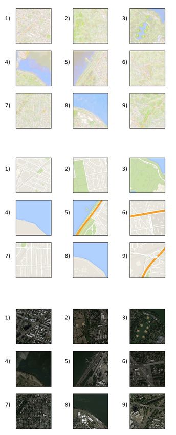
Figure 1: A grid comparing the the satellite images from Google Earth Engine along with the
corresponding Google Maps tile

     2. Adding a pixel-wise reconstruction loss in addition to the GAN loss which measures the
        pixel-wise normed distance between the generated maps and the real map which is available
        at training time.
     3. Adding a style reconstruction loss to the losses described in the previous item. The style
        reconstruction loss has the same mathematical structure as the style loss in neural style trans-
        fer Gatys, Ecker, and Bethge (2015). This loss emphasizes not only pixel-wise coherence
        but also makes sure that the corrlation between a pixels and their neighbors have the same
        characteristics as the real map.
     4. Experimenting with performance using L1 versus L2 norm for determining the recon-
        struction loss. The different norm operations have been known to aid training depending
        on the task. While CycleGAN (Zhu et al. (2018)) benefits from the L1 penalty in its
        cycle-consistency loss, we observe that the L2 norm performs better for our task.
     5. While it is straightforward to condition the output of the generator of a GAN to a given input,
        it is not clear how to condition the discriminator. We try two approaches. The first approach
        is to use the compressed and encoded version of the satellite image and concatenate it to the
        prefinal layer of the output of the discriminator before passing it through a final set of layers
        to obtain the discriminator’s decision probability. The other approach is to concatenate
        the satellite image to the real or the fake image along the channel axis. This allows the
        convolution filters to have access to the full satellite image while making a decision on how
        realistic the generated maps are. This approach therefore totally bi-passes the need for an
        encoder.
     6. Using a RealNVP generator instead of the standard convolutional generator. RealNVP is a
        bijective model and thus allows us to translate very efficiently from the map image domain
        to the satellite image domain and the vice versa.
     7. While we are continuing to work on increasing the accuracy of the model, one challenge
        has been the coarse resolution of the data which upper-bounds the quality of the results of
        our model. Nevertheless, as will be seen in the results, the generated map is more accurate
        in the features it produces since the generator architecture demands a pixel-wise image
        translation/pixel-wise coloring. For example, if we look at tile number 6 in figure 6, we
        see that the generated map is more accurate and has more features than the real map when
        compared with the available satellite image.
     8. To the best of our knowledge, ours is the first model to incorporate a reconstruction loss
        (for pixel-wise accuracy) and a style loss (to reduce high frequency artifacts) in addition
        to the GAN loss (a feature-wise learnt similarity metric or content loss similar to the ideas
        presented in Gatys, Ecker, and Bethge (2015) and Larsen, Sønderby, and Winther (2015))
        for the task of generating the standard layer of the map from a satellite image.

                                                   4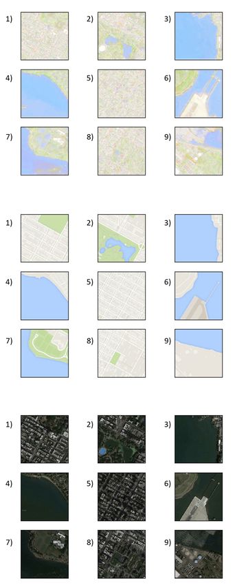
4.2   Evaluation Method

Given that GANs are not evaluated by tracking likelihoods, most of our evaluation will be qualitative.
I.E. to see if our models learned the distribution of well, we can sample new satellite images,
generate maps for them, and perform a small experiment to see whether humans and can differentiate
between the real and generated maps/topographies. However, we do have "ground truths" for the map
translation task and can also track image similarity indexes. Some similarity indexes include L1 and
L2 reconstruction losses. We track a combination of L2 loss and style reconstruction loss and see an
improvement over training. We created three high level models based on three different philosophies
which are described below.

4.3   Model 1: Conditional GAN

One way to think about our task is that want the Generator, instead of generating a map image
based random noise, to generate a map image based on information in the satellite tile. Creating a
lower dimensional representation of the satellite images to feed into the generator will allow could
afford several very nice tasks such as (1) Analyze how the generator treats this lower dimensional
space, hopefully finding disentangled representations (2) More naturally interpolate between different
satellite images in this space (3) More naturally add custom features and hope that the generator uses
them in order to later interpolate them and create new maps with tweaked high level attributes (ie.
population density in the region, the lat/long region, the city, the year, etc.). Mirza and Osindero
(2014) was able to generate encouraging results for GAN Generators trained on feature vectors, and so
model 1 is constructed to extract the useful information from the satellite image into a feature vector,
then pass it to a generator. 64x64x3 are passed through a deep convolutional network (Encoder) to
create 100 or 512 long embeddings. These embeddings are either appended or element wise added
Gaussian noise. Then a convolutional Generator is provided these embedding to generate the 64x64x3
map. The Encoder and Generator are trained jointly with a convolutional Discriminator using the
standard GAN discriminator loss. The standard GAN non-saturating generator loss is used for the
generator loss. Given we know the correct fake-real map pairs, a reconstruction loss can be computed
as the norm of the difference between the images. Figure 2 shows the model architecture.
Discriminator loss
                       max Ex∼pReal [log D (x)] + Ez∼pNoise [log(1 − D(G(z)))]                      (1)
                        D

Generator loss
                                     min −Ez∼pNoise [log D(G(z))]                                   (2)
                                      G

Reconstruction loss
                                          ||Mfake − Mreal ||2                                       (3)
Embedding the input in a lower dimensional vector and appending noise was inspired by Deng,
Zhu, and Newsam (2018). Using deep fully convolutional networks was motivated by Radford,
Metz, and Chintala (2015). We experimented with different embeddings such as 100 and 512 long
vectors, different ways to add noise (appending vs adding element wise), different relative lengths
and magnitudes of the noise vectors, and both L1 and L2 reconstruction losses.

4.4   Model 2: Conditional GAN without Encoder and with reconstruction loss

The second approach for satellite to image translation involves treating it as a cross between an image
generation and a pixel level discrimination between the different map color classes (gray for road,
green for vegetation, blue for water, etc.). We could use a U-net for this model, as is done by Isola et
al. (2016), which uses a U-net with a PathGAN discriminator (the PatchGAN penalizes textures of the
output that are too different from those in ground truths. However, the simplest model is just a series
of convolutions which give every pixel an effective receptive field around it’s position in the original
image. As such we came up with the architecture shown in Figure 3 which does not include an
encoder. We also added a reconstruction loss (equation 3). We noticed that some of the details from
the satellite images are transferred over to the generated maps, so we added a style transfer loss. The
style-transfer loss can be written as follows where Gij represents the gram-matrix for the generated
image and Aij is the gram-matrix for the ground truth maps image. The gram-matrix represent the

                                                   5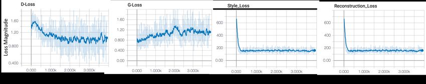
Reconstruction Loss

                                                Gaussian
                                                 Noise

                                                                      512
                                                                                   Generator             Generated
                64 x 64 x 3                                                                                Map
                                                            512             1024

             Satellite Image                                                                              64 x 64 x 3
                                                             Embedding
                                            Encoder

                                                                                                   512
                                Real
                                Map
                                                                                                                  PReal

                                                                                                 512

                              64 x 64 x 3                                                  Discriminator

Figure 2: A schematic of the baseline GeoGAN model. The generation of the map is conditioned
on the satellite image along with some optional noise. The discriminator is also supplied with the
conditional information from the satellite image embedding. One architecture we used is as follows
(with c(x x y x z) sn referring to a convolution with a z filters of size x ∗ y and a stride of n, cT(x x
y x z) sn is the same with transposed convolutions, and lr referring to a a leaky rely layer): Encoder:
input=batchx64x64x3; layers = c(3x3x1024) s2, lr, c(3x3x512) s2, lr c(3x3x256) s2, lr, c(3x3x128) s2,
lr, c(4x4x512) s1, batchnorm, lr; output= c(batchx1x1x512) Noise: input=batchx64x64x3; element
wise add noise; output=batchx64x64x3 Generator: input=batchx1x1x512; layers cT(4x4x1024) s1,
lr, cT(8x8x512) s2, lr, cT(3x3x128) s2, lr, cT(3x3x32) s2, lr, cT(3x3x64) s2; output=batchx64x64x3
Discriminator: input=batchx64x64x3; c(3x3x128) s2, lr, c(3x3x256) s2, lr, c(3x3x512) s2, lr,
c(3x3x1024) s2, lr, c(4x4x512) s1, lr, concatenate 512 activation units with embedding of sat image,
fully connected layer with 512 outputs, lr, fully connected layer, sigmoid. Convolution padding is
omitted for brevity.

inner-product of the image F . N represents the amount of channels and M is the product of the
height and width of the images.
Style loss                                            X
                                              Gij =        Fik Fjk
                                                      k
                                                                                                        (4)
                                                    1                  2
                                    Lstyle =              (Gij − Aij )
                                                4N 2 M 2
In the original style transfer paper, this style loss is calculated as a sum over the activation of all the
layers. However, in our case we don’t have a completely trained model to extract style from, so we
suffice with taking the style loss of the map images directly.

4.5   Model 3: Real NVP

Zhu et al. (2018) showed impressive results Zhu et al. (2018) on satellite to map translation using
convolutional Cycle GANS. In their paper, the networks for the forwards and backwards (satellite
→ map, and map→satellite) were trained jointly using a reconstruction loss. Flow models have the
benefit of being invertible so they make natural fits for cycle GANs. In more detail, a flow model and
it’s inverse implicitly incorporates a direct reconstruction without having to make the model learn
such through adding additional loss penalties or a cycle-consistency loss. The forward direction is
simply the bijection from a noise distribution to the image, and the backward direction will be its
inverse. Because the forward and backward operations are exact inverses of each other, there should

                                                                  6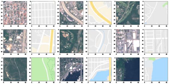
Reconstruction
                                                   Loss
                                                     +
                                                Style Loss                        PReal

                                                               Generated
              256 x 256 x 3                                      Map                      Discriminator

           Satellite Image                                     256 x 256 x 3

                                              Generator

                                 Real
                                 Map                                           Concatenate
                                                                                  Along
                                                                                Channels
                                                                                   Axis

                              256 x 256 x 3

Figure 3: A schematic of the GeoGAN model without encoding. The generation of the map is
conditioned on the entire satellite image. Each input to the discriminator is 256 x 256 x 6, which
is a satellite image concatenated with either the real or generated map along the channel axis. A
more detailed description of our architecture is below: Generator: To give two different sizes of
receptive fields a chance to compete for weights in each layer, each convectional layer is a channel
wise concatenation of n (3x3) convolutional filters and n (5x5) convolutional filters followed by a
leaky ReLu. For the first four layers, n is equal to 300,150,60, and 20. The last layer is a transposed
3x3 convolution bringing the last 40 layers to 3 followed by a tanh.Discriminator: The first four
layers in the discriminator are 3x3 convolutions with stride two and 128, 256, 512, 768 and 1024
filters respectively. (All followed by leaky ReLu layers). The last layer is a 4x4 convolution followed
by sigmoid.

be no reconstruction loss, therefore the loss function should be the sum of the two discriminator’s
losses. We chose RealNVP for our flow model because it is has shown good performance on more
complicated real world images such a faces and is not as hard to train as Glow Kingma and Dhariwal
(2018). We attempt creating the RealNVP architecture similarly to Dinh, Sohl-Dickstein, and Bengio
(2016) by first using 2 bijections with checkerboard masking followed by another 2 bijections
channel-wise masking. The different masking operations are to vary which half of the total pixels get
transformed by the RealNVP bijection. All bijections use the RealNVP bijection implementation in
Tensorflow with two FC layers of 512 units along with batchnorm. This method differs as a more
simple implementation than the full RealNVP that uses a residual based network. It should also
be noted that the RealNVP model used in the original paper trains through maximum likelihood
optimization, which is what a GAN based approach tends to avoid (Dinh, Sohl-Dickstein, and Bengio
(2016)).

5     Results

5.1   Conditional GAN with encoder

While this model performed well on our MNIST sanity check (see figure 8 in the appendix) it failed
to train well on our satellite images dataset. The training losses would saturate for both the Generator
and Discriminator (see figure 4). The samples were also bad quality. This seemed to always be the
case when we tried changing the noise levels noise at 0%, 10%, and 50% noise.

                                                               7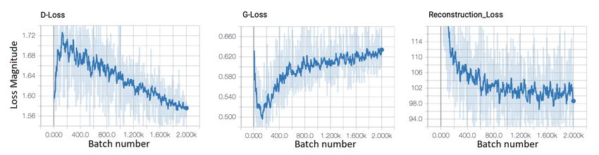
Figure 4: The generator, discriminator and reconstruction losses of the conditional GAN with the
encoder and only the reconstruction loss trained on the dataset we generated. The discriminator is
very quickly learning to tell real maps from fake maps and the Generator and discriminator losses
saturate at their current points.

Figure 5: Loss curves over 14 epochs of the GAN without an encoder trainded with GAN, recon-
struction and style loss on the CycleGAN dataset. The image quality improves after 3-4 epochs when
the reconstruction and style losses start to plateau.

5.2   Conditional GAN without encoder

This model performed, by far, the best, especially when trained with the reconstruction and style
losses. The training curves for one of our runs is shown in figure 5. Some examples of maps generated
using this model trained on the CycleGAN dataset can be found in figure 6. More samples can be
found in the appendix. This data is all from the test, not training dataset and was randomly sampled
(not hand selected).

5.3   RealNVP

We ran a sanity check on our RealNVP based model by running it through MNIST. However, it seems
that the model suffers from mode collapse as the generate example all tend to match the same digit,
in this case the digit 9. A figure of this is in the appendix. We suspect that this is due to the model
requiring more complexity or ill-posing the training objective. Not passing the MNIST sanity-check
lead us terminate moving forward with the idea of using a RealNVP generator 8. We notice the loss
curves for this type of model also resemble how a GAN training on MNIST should look like.

6     Analysis

6.1   Baseline Conditional GAN

The conditional GAN with encoder was not able to generate convincing maps despite our search over
hyperparameters such as size of the encoded vector, varying degrees and types of noise and slightly
varying architectures. It might be that creating a meaningful embedding and generating realistic
images is too demanding of a task for the Generator. We tried techniques such as having more training
updates for the generator for each update of the discriminator to little success. It is possible that if we
pretrained the encoder as part of an auto-encoder before plugging it in to the generator it would have
better odds of success. It would be great to get the autoencoder working because then we could more
naturally interpolate in this latent space to generate different maps as well as add custom features to
this encoding in order to generate new maps.

                                                    8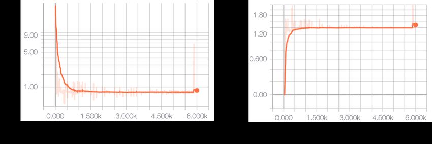
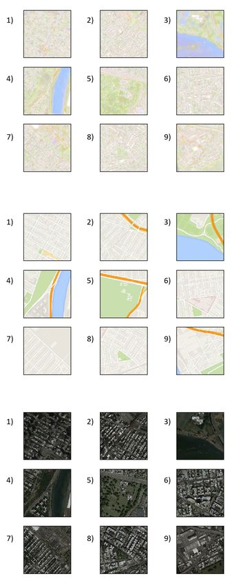
Figure 6: A sample of 9 maps generated by GeoGAN - Model 3 trained on the CycleGAN dataset.

                                             9
6.2 Conditional GAN Without Encoder
As is seen from the figures, the model trains well and converges by the end of the tenth epoch.
The generator and the discriminator are only three layers deep and preliminary investigations by
increasing the depth of the discriminator and generator show that the loss values are lower.
6.3 RealNVP
The suspected mode collapse of the model might be due to lack of complexity since we use an FC
approach to create the shift and scale function of the bisections. However, experiments with even
adding more hidden layers or doubling the size of the two hidden layers quickly resulted in numerical
overflow when applying the gradient updates. Additionally, the true RealNVP paper implementation
used a convolutional and residual network approach for these functions for more complicated data
like faces. However, there wasn’t a way to add this complexity with the Tensorflow API function
that applied the RealNVP transformations. Another point of conflict that might be happening is
that we trained the RealNVP generator through the GAN loss functions. This is different than how
flow models are are trained in practice, which is through maximum likelihood estimation on the
training data. Recall that the point of the GAN generative model approach was to avoid thinking
about likelihoods and instead let the adversarial examples be the training signal. Thus, it could be
that the RealNVP generator learned to generate samples that might fool the discriminator at times by
creating the same digit out of the noise inputs. The model however didn’t learn diversity since the
gradient wasn’t computed with respect to the likelihood of the RealNVP generating samples from the
training set. Mixing likelihood maximization and GAN based training might be an area of further
research to validate that such a hybrid approach is possible.
6.4 Data
Our best results were achieved while training on the CycleGAN maps dataset Zhu et al. (2018); Park
(2018) as opposed to our generated data-set because the satellite imagery was much higher resolution
and more free from clouds. It would appear that satellite imagery resolutions of 10m2 per pixel does
not yield great results. Our model is often confused by water vs vegetation (as both are dark blues
and greens colors) and sometimes reflections on the surface of water. Therefore we think that adding
IR or other bands (which are present in our generated dataset).
7 Conclusion
In conclusion, we demonstrate a viable model for generating maps (the GAN with reconstruction
and style transfer losses and no encoder). The results shown have no hyperparameter search and
are only trained on 15 epochs, we believe that with more training time we can achieve even more
realistic results. Future work could also include training on more bands, such as IR to help the map
distinguish between visually ambiguous regions such as lakes and vegetation. These additional bands
exist in the data we pulled from google earth engine. We also provide code to generate new datasets
from earth engine and google maps API. While the 10m resolution images from sentinel 2 do no
train well, our data gathering streams can pull any data from google earth engine including satellite
imagery, elevation data, thermal data, and more. A dataset for any translation between those domains
or between maps is able to be pulled.
References
Arjovsky, M.; Chintala, S.; and Bottou, L. 2017. Wasserstein Generative Adversarial Networks.
Proceedings of the 34th International Conference on Machine Learning, Sydney, Australia, PMLR
70, 2017.
Chan, C.; Ginosar, S.; Zhou, T.; and Efros, A. A. 2018. Everybody dance now. arXiv preprint
arXiv:1808.07371.
Costea, D.; Marcu, A.; Slusanschi, E.; and Leordeanu, M. 2017. Creating Roadmaps in Aerial
Images with Generative Adversarial Networks and Smoothing-based Optimization. ICCV 2017
Workshops.
10Demir, I.; Koperski, K.; Lindenbaum, D.; Pang, G.; Huang, J.; Basu, S.; Hughes, F.; Tuia, D.; and
Raskar, R. 2018. DeepGlobe 2018: A Challenge to Parse the Earth through Satellite Images.
arXiv:1805.06561v1.
Deng, X.; Zhu, Y.; and Newsam, S. 2018. What Is It Like Down There? Generating Dense
Ground-Level Views and Image Features From Overhead Imagery Using Conditional Generative
Adversarial Networks. SIGSPATIAL 18, November 2018, Seattle, Washington USA.
Dinh, L.; Sohl-Dickstein, J.; and Bengio, S. 2016. Density estimation using real NVP. CoRR
abs/1605.08803.
Dunnmon, J.; Ganguli, S.; Hau, D.; and Husic, B. 2019. Predicting us state-level agricultural
sentiment as a measure of food security with tweets from farming communities. arXiv preprint
arXiv:1902.07087.
Engine, G. E. 2018. Sentinel2 data copernicus:s2 on google earth engine.
https://developers.google.com/earth-engine/datasets/catalog/COPERNICUS, Online: Ac-
cessed 2018-10-24.
Ganguli, S.; Dunnmon, J.; and Hau, D. 2019. Predicting food security outcomes using convolutional
neural networks (cnns) for satellite tasking. arXiv preprint arXiv:1902.05433.
Gatys, L. A.; Ecker, A. S.; and Bethge, M. 2015. A Neural Algorithm of Artistic Style.
arXiv:1508.06576.
Goodfellow, I. J.; Pouget-Abadie, J.; Mirza, M.; Xu, B.; Warde-Farley, D.; Ozair, S.; Courville, A.;
and Bengio, Y. 2014. Generative Adversarial Networks. arXiv:1406.2661.
Gulrajani, I.; Ahmed, F.; Arjovsky, M.; Dumoulin, V.; and Courville, A. 2017. Improved Training of
Wasserstein GANs. arXiv:1704.00028.
Isola, P.; Zhu, J.-Y.; Zhou, T.; and Efros, A. A. 2016. Image-to-Image Translation with Conditional
Adversarial Networks. ArXiv:1611.07004.
Kingma, D. P., and Dhariwal, P. 2018. Glow: Generative Flow with Invertible 1x1 Convolutions.
arXiv:1807.03039.
Larsen, A. B. L.; Sønderby, S. K.; and Winther, O. 2015. Autoencoding beyond pixels using a
learned similarity metric. CoRR abs/1512.09300.
Mirza, M., and Osindero, S. 2014. Conditional GANs. arXiv:1411.1784.
Park, T. 2018. Satellite to Maps Dataset. https://people.eecs.berkeley.edu/ tae-
sung_park/CycleGAN/datasets/maps.zip, Online: Accessed 11-Dec-2018.
Perez, A.; Ganguli, S.; Ermon, S.; Azzari, G.; Burke, M.; and Lobell, D. 2019. Semi-supervised mul-
titask learning on multispectral satellite images using wasserstein generative adversarial networks
(gans) for predicting poverty. arXiv preprint arXiv:1902.11110.
Radford, A.; Metz, L.; and Chintala, S. 2015. Unsupervised Representation Learning with Deep
Convolutional Generative Adversarial Networks. arXiv:1511.06434.
Xu, C., and Zhao, B. 2018. Satellite Image Spoofing: Creating Remote Sensing Dataset with
Generative Adversarial Networks. 10th International Conference on Geographic Information
Science.
Zhu, J.-Y.; Park, T.; Isola, P.; and Efros, A. A. 2018. Unpaired image-to-image translation using
cycle-consistent adversarial networks. arXiv:1703.10593.
11A MNIST Sanity Checks
As a sanity check for our baseline architecture, we train our model on the MNIST dataset. The
discriminator and generator loss over time in this case is shown in figure 7. A sample of the generated
images at epoch 20 from this training and an example output of training the NVP model is shown in
figure 8.
Figure 7: The discriminator and generator loss of the GeoGAN encoder trained on MNIST to evaluate
whether the model can capture a simple distribution like handwritten digits.
Figure 8: Generated samples from the GeoGAN at epoch 20 when trained on the MNIST dataset
on the left and those from RealNVP-based generator model at 6 epochs of training on the MNIST
dataset. Each small tile is a different sample. There is a clear indication of mode collapse with the
RealNVP generator which we were not able to fix.
12B Demonstration: Seasonality Effects are Encoded by Using Four Pairs
(Summer, Fall, Winter, Spring) of Satellite Images for the Same Map:
Figure 9: A grid comparing the the satellite images from Google Earth Engine of the same tile at
different seasons (four seasons) along with the corresponding Google Maps tile.
13C Additional Samples from Trained GeoGAN (Model 3):
Figure 10: A sample of 9 maps generated by GeoGAN - Model 3 trained on the CycleGAN dataset.
14Figure 11: A sample of 9 maps generated by GeoGAN - Model 3 trained on the CycleGAN dataset.
15Figure 12: A sample of 9 maps generated by GeoGAN - Model 3 trained on the CycleGAN dataset.
16Figure 13: A sample of 9 maps generated by GeoGAN - Model 3 trained on the CycleGAN dataset.
17Figure 14: A sample of 9 maps generated by GeoGAN - Model 3 trained on the CycleGAN dataset.
18You can also read