A Discriminatively Trained, Multiscale, Deformable Part Model
←
→
Page content transcription
If your browser does not render page correctly, please read the page content below
A Discriminatively Trained, Multiscale, Deformable Part Model

     Pedro Felzenszwalb                              David McAllester                                         Deva Ramanan
    University of Chicago                 Toyota Technological Institute at Chicago                             UC Irvine
    pff@cs.uchicago.edu                             mcallester@tti-c.org                                   dramanan@ics.uci.edu

                            Abstract

   This paper describes a discriminatively trained, multi-
scale, deformable part model for object detection. Our sys-
tem achieves a two-fold improvement in average precision
over the best performance in the 2006 PASCAL person de-
tection challenge. It also outperforms the best results in the
2007 challenge in ten out of twenty categories. The system
relies heavily on deformable parts. While deformable part
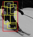
models have become quite popular, their value had not been                   Figure 1. Example detection obtained with the person model. The
demonstrated on difficult benchmarks such as the PASCAL                      model is defined by a coarse template, several higher resolution
                                                                             part templates and a spatial model for the location of each part.
challenge. Our system also relies heavily on new methods
for discriminative training. We combine a margin-sensitive
approach for data mining hard negative examples with a                       object categories. Figure 1 shows an example detection ob-
formalism we call latent SVM. A latent SVM, like a hid-                      tained with our person model.
den CRF, leads to a non-convex training problem. How-
                                                                                 The notion that objects can be modeled by parts in a de-
ever, a latent SVM is semi-convex and the training prob-
                                                                             formable configuration provides an elegant framework for
lem becomes convex once latent information is specified for
                                                                             representing object categories [1–3, 6, 10, 12, 13, 15, 16, 22].
the positive examples. We believe that our training meth-
                                                                             While these models are appealing from a conceptual point
ods will eventually make possible the effective use of more
                                                                             of view, it has been difficult to establish their value in prac-
latent information such as hierarchical (grammar) models
                                                                             tice. On difficult datasets, deformable models are often out-
and models involving latent three dimensional pose.
                                                                             performed by “conceptually weaker” models such as rigid
                                                                             templates [5] or bag-of-features [23]. One of our main goals
1. Introduction                                                              is to address this performance gap.
    We consider the problem of detecting and localizing ob-                      Our models include both a coarse global template cov-
jects of a generic category, such as people or cars, in static               ering an entire object and higher resolution part templates.
images. We have developed a new multiscale deformable                        The templates represent histogram of gradient features [5].
part model for solving this problem. The models are trained                  As in [14, 19, 21], we train models discriminatively. How-
using a discriminative procedure that only requires bound-                   ever, our system is semi-supervised, trained with a max-
ing box labels for the positive examples. Using these mod-                   margin framework, and does not rely on feature detection.
els we implemented a detection system that is both highly                    We also describe a simple and effective strategy for learn-
efficient and accurate, processing an image in about 2 sec-                  ing parts from weakly-labeled data. In contrast to computa-
onds and achieving recognition rates that are significantly                  tionally demanding approaches such as [4], we can learn a
better than previous systems.                                                model in 3 hours on a single CPU.
    Our system achieves a two-fold improvement in average                        Another contribution of our work is a new methodology
precision over the winning system [5] in the 2006 PASCAL                     for discriminative training. We generalize SVMs for han-
person detection challenge. The system also outperforms                      dling latent variables such as part positions, and introduce a
the best results in the 2007 challenge in ten out of twenty                  new method for data mining “hard negative” examples dur-
                                                                             ing training. We believe that handling partially labeled data
    This material is based upon work supported by the National Science       is a significant issue in machine learning for computer vi-
Foundation under Grant No. 0534820 and 0535174.                              sion. For example, the PASCAL dataset only specifies a

                                                                         1
bounding box for each positive example of an object. We
treat the position of each object part as a latent variable. We
also treat the exact location of the object as a latent vari-
able, requiring only that our classifier select a window that
has large overlap with the labeled bounding box.
A latent SVM, like a hidden CRF [19], leads to a non-
convex training problem. However, unlike a hidden CRF,
a latent SVM is semi-convex and the training problem be-
comes convex once latent information is specified for the
positive training examples. This leads to a general coordi-
nate descent algorithm for latent SVMs.
System Overview Our system uses a scanning window
approach. A model for an object consists of a global “root”
filter and several part models. Each part model specifies a
spatial model and a part filter. The spatial model defines a
Image pyramid HOG feature pyramid
set of allowed placements for a part relative to a detection
window, and a deformation cost for each placement. Figure 2. The HOG feature pyramid and an object hypothesis de-
fined in terms of a placement of the root filter (near the top of the
The score of a detection window is the score of the root
pyramid) and the part filters (near the bottom of the pyramid).
filter on the window plus the sum over parts, of the maxi-
mum over placements of that part, of the part filter score on
the resulting subwindow minus the deformation cost. This detection window. Finer scale features are captured by part
is similar to classical part-based models [10, 13]. Both root templates that can be moved with respect to the detection
and part filters are scored by computing the dot product be- window. The spatial model for the part locations is equiv-
tween a set of weights and histogram of gradient (HOG) alent to a star graph or 1-fan [3] where the coarse template
features within a window. The root filter is equivalent to a serves as a reference position.
Dalal-Triggs model [5]. The features for the part filters are
computed at twice the spatial resolution of the root filter. 2.1. HOG Representation
Our model is defined at a fixed scale, and we detect objects
by searching over an image pyramid. We follow the construction in [5] to define a dense repre-
In training we are given a set of images annotated with sentation of an image at a particular resolution. The image
bounding boxes around each instance of an object. We re- is first divided into 8x8 non-overlapping pixel regions, or
duce the detection problem to a binary classification prob- cells. For each cell we accumulate a 1D histogram of gra-
lem. Each example x is scored by a function of the form, dient orientations over pixels in that cell. These histograms
fβ (x) = maxz β · Φ(x, z). Here β is a vector of model pa- capture local shape properties but are also somewhat invari-
rameters and z are latent values (e.g. the part placements). ant to small deformations.
To learn a model we define a generalization of SVMs that The gradient at each pixel is discretized into one of nine
we call latent variable SVM (LSVM). An important prop- orientation bins, and each pixel “votes” for the orientation
erty of LSVMs is that the training problem becomes convex of its gradient, with a strength that depends on the gradient
if we fix the latent values for positive examples. This can magnitude. For color images, we compute the gradient of
be used in a coordinate descent algorithm. each color channel and pick the channel with highest gradi-
In practice we iteratively apply classical SVM training to ent magnitude at each pixel. Finally, the histogram of each
triples (hx1 , z1 , y1 i, . . ., hxn , zn , yn i) where zi is selected cell is normalized with respect to the gradient energy in a
to be the best scoring latent label for xi under the model neighborhood around it. We look at the four 2 × 2 blocks
learned in the previous iteration. An initial root filter is of cells that contain a particular cell and normalize the his-
generated from the bounding boxes in the PASCAL dataset. togram of the given cell with respect to the total energy in
The parts are initialized from this root filter. each of these blocks. This leads to a vector of length 9 × 4
representing the local gradient information inside a cell.
2. Model We define a HOG feature pyramid by computing HOG
features of each level of a standard image pyramid (see Fig-
The underlying building blocks for our models are the ure 2). Features at the top of this pyramid capture coarse
Histogram of Oriented Gradient (HOG) features from [5]. gradients histogrammed over fairly large areas of the input
We represent HOG features at two different scales. Coarse image while features at the bottom of the pyramid capture
features are captured by a rigid template covering an entire finer gradients histogrammed over small areas.
22.2. Filters of each part relative to the root (the spatial term),
Filters are rectangular templates specifying weights for n
X n
X
subwindows of a HOG pyramid. A w by h filter F is a Fi · φ(H, pi ) + ai · (x̃i , ỹi ) + bi · (x̃2i , ỹi2 ), (1)
vector with w × h × 9 × 4 weights. The score of a filter is i=0 i=1
defined by taking the dot product of the weight vector and where (x̃i , ỹi ) = ((xi , yi ) − 2(x, y) + vi )/si gives the lo-
the features in a w × h subwindow of a HOG pyramid. cation of the i-th part relative to the root location. Both x̃i
The system in [5] uses a single filter to define an object and ỹi should be between −1 and 1.
model. That system detects objects from a particular class There is a large (exponential) number of placements for
by scoring every w × h subwindow of a HOG pyramid and a model in a HOG pyramid. We use dynamic programming
thresholding the scores. and distance transforms techniques [9, 10] to compute the
Let H be a HOG pyramid and p = (x, y, l) be a cell in best location for the parts of a model as a function of the
the l-th level of the pyramid. Let φ(H, p, w, h) denote the root location. This takes O(nk) time, where n is the number
vector obtained by concatenating the HOG features in the of parts in the model and k is the number of cells in the
w × h subwindow of H with top-left corner at p. The score HOG pyramid. To detect objects in an image we score root
of F on this detection window is F · φ(H, p, w, h). locations according to the best possible placement of the
Below we use φ(H, p) to denote φ(H, p, w, h) when the parts and threshold this score.
dimensions are clear from context. The score of a placement z can be expressed in terms
of the dot product, β · ψ(H, z), between a vector of model
2.3. Deformable Parts parameters β and a vector ψ(H, z),
Here we consider models defined by a coarse root filter β = (F0 , . . . , Fn , a1 , b1 . . . , an , bn ).
that covers the entire object and higher resolution part filters
ψ(H, z) = (φ(H, p0 ), φ(H, p1 ), . . . φ(H, pn ),
covering smaller parts of the object. Figure 2 illustrates a
placement of such a model in a HOG pyramid. The root fil- x̃1 , ỹ1 , x̃21 , ỹ12 , . . . , x̃n , ỹn , x̃2n , ỹn2 , ).
ter location defines the detection window (the pixels inside
We use this representation for learning the model parame-
the cells covered by the filter). The part filters are placed
ters as it makes a connection between our deformable mod-
several levels down in the pyramid, so the HOG cells at that
els and linear classifiers.
level have half the size of cells in the root filter level.
On interesting aspect of the spatial models defined here
We have found that using higher resolution features for
is that we allow for the coefficients (ai , bi ) to be negative.
defining part filters is essential for obtaining high recogni-
This is more general than the quadratic “spring” cost that
tion performance. With this approach the part filters repre-
has been used in previous work.
sent finer resolution edges that are localized to greater ac-
curacy when compared to the edges represented in the root
filter. For example, consider building a model for a face.
3. Learning
The root filter could capture coarse resolution edges such as The PASCAL training data consists of a large set of im-
the face boundary while the part filters could capture details ages with bounding boxes around each instance of an ob-
such as eyes, nose and mouth. ject. We reduce the problem of learning a deformable part
The model for an object with n parts is formally defined model with this data to a binary classification problem. Let
by a root filter F0 and a set of part models (P1 , . . . , Pn ) D = (hx1 , y1 i, . . . , hxn , yn i) be a set of labeled exam-
where Pi = (Fi , vi , si , ai , bi ). Here Fi is a filter for the i-th ples where yi ∈ {−1, 1} and xi specifies a HOG pyramid,
part, vi is a two-dimensional vector specifying the center for H(xi ), together with a range, Z(xi ), of valid placements
a box of possible positions for part i relative to the root po- for the root and part filters. We construct a positive exam-
sition, si gives the size of this box, while ai and bi are two- ple from each bounding box in the training set. For these ex-
dimensional vectors specifying coefficients of a quadratic amples we define Z(xi ) so the root filter must be placed to
function measuring a score for each possible placement of overlap the bounding box by at least 50%. Negative exam-
the i-th part. Figure 1 illustrates a person model. ples come from images that do not contain the target object.
A placement of a model in a HOG pyramid is given by Each placement of the root filter in such an image yields a
z = (p0 , . . . , pn ), where pi = (xi , yi , li ) is the location of negative training example.
the root filter when i = 0 and the location of the i-th part Note that for the positive examples we treat both the part
when i > 0. We assume the level of each part is such that a locations and the exact location of the root filter as latent
HOG cell at that level has half the size of a HOG cell at the variables. We have found that allowing uncertainty in the
root level. The score of a placement is given by the scores root location during training significantly improves the per-
of each filter (the data term) plus a score of the placement formance of the system (see Section 4).
33.1. Latent SVMs negative examples at a time. Instead, it is common to con-
struct training data consisting of the positive instances and
A latent SVM is defined as follows. We assume that each
“hard negative” instances, where the hard negatives are data
example x is scored by a function of the form,
mined from the very large set of possible negative examples.
fβ (x) = max β · Φ(x, z), (2) Here we describe a general method for data mining ex-
z∈Z(x) amples for SVMs and latent SVMs. The method iteratively
where β is a vector of model parameters and z is a set solves subproblems using only hard instances. The innova-
of latent values. For our deformable models we define tion of our approach is a theoretical guarantee that it leads
Φ(x, z) = ψ(H(x), z) so that β · Φ(x, z) is the score of to the exact solution of the training problem defined using
placing the model according to z. the complete training set. Our results require the use of a
In analogy to classical SVMs we would like to train β margin-sensitive definition of hard examples.
from labeled examples D = (hx1 , y1 i, . . . , hxn , yn i) by The results described here apply both to classical SVMs
optimizing the following objective function, and to the problem defined by Step 2 of the coordinate de-
scent algorithm for latent SVMs. We omit the proofs of the
n
X theorems due to lack of space. These results are related to
β ∗ (D) = argmin λ||β||2 + max(0, 1 − yi fβ (xi )). (3) working set methods [17].
β i=1
We define the hard instances of D relative to β as,
By restricting the latent domains Z(xi ) to a single choice,
M (β, D) = {hx, yi ∈ D | yfβ (x) ≤ 1}. (4)
fβ becomes linear in β, and we obtain linear SVMs as a
special case of latent SVMs. Latent SVMs are instances of That is, M (β, D) are training examples that are incorrectly
the general class of energy-based models [18]. classified or near the margin of the classifier defined by β.
We can show that β ∗ (D) only depends on hard instances.
3.2. Semi-Convexity
Theorem 1. Let C be a subset of the examples in D. If
Note that fβ (x) as defined in (2) is a maximum of func- M (β ∗ (D), D) ⊆ C then β ∗ (C) = β ∗ (D).
tions each of which is linear in β. Hence fβ (x) is convex
in β. This implies that the hinge loss max(0, 1 − yi fβ (xi )) This implies that in principle we could train a model us-
is convex in β when yi = −1. That is, the loss function is ing a small set of examples. However, this set is defined in
convex in β for negative examples. We call this property of terms of the optimal model β ∗ (D).
the loss function semi-convexity. Given a fixed β we can use M (β, D) to approximate
Consider an LSVM where the latent domains Z(xi ) for M (β ∗ (D), D). This suggests an iterative algorithm where
the positive examples are restricted to a single choice. The we repeatedly compute a model from the hard instances de-
loss due to each positive example is now convex. Combined fined by the model from the last iteration. This is further
with the semi-convexity property, (3) becomes convex in β. justified by the following fixed-point theorem.
If the labels for the positive examples are not fixed we Theorem 2. If β ∗ (M (β, D)) = β then β = β ∗ (D).
can compute a local optimum of (3) using a coordinate de-
scent algorithm: Let C be an initial “cache” of examples. In practice we
can take the positive examples together with random nega-
1. Holding β fixed, optimize the latent values for the pos- tive examples. Consider the following iterative algorithm:
itive examples zi = argmaxz∈Z(xi ) β · Φ(x, z).
1. Let β := β ∗ (C).
2. Holding {zi } fixed for positive examples, optimize β
2. Shrink C by letting C := M (β, C).
by solving the convex problem defined above.
3. Grow C by adding examples from M (β, D) up to a
It can be shown that both steps always improve or maintain
memory limit L.
the value of the objective function in (3). If both steps main-
tain the value we have a strong local optimum of (3), in the Theorem 3. If |C| < L after each iteration of Step 2, the
sense that Step 1 searches over an exponentially large space algorithm will converge to β = β ∗ (D) in finite time.
of latent labels for positive examples while Step 2 simulta-
neously searches over weight vectors and an exponentially 3.4. Implementation details
large space of latent labels for negative examples. Many of the ideas discussed here are only approximately
implemented in our current system. In practice, when train-
3.3. Data Mining Hard Negatives
ing a latent SVM we iteratively apply classical SVM train-
In object detection the vast majority of training exam- ing to triples hx1 , z1 , y1 i, . . ., hxn , zn , yn i where zi is se-
ples are negative. This makes it infeasible to consider all lected to be the best scoring latent label for xi under the
4model trained in the previous iteration. Each of these triples
leads to an example hΦ(xi , zi ), yi i for training a linear clas-
sifier. This allows us to use a highly optimized SVM pack-
age (SVMLight [17]). On a single CPU, the entire training
process takes 3 to 4 hours per object class in the PASCAL
datasets, including initialization of the parts.
Root Filter Initialization: For each category, we auto-
matically select the dimensions of the root filter by looking
at statistics of the bounding boxes in the training data.1 We
train an initial root filter F0 using an SVM with no latent
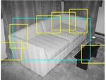
variables. The positive examples are constructed from the Figure 3. The image on the left shows the optimization of the la-
unoccluded training examples (as labeled in the PASCAL tent variables for a positive example. The dotted box is the bound-
data). These examples are anisotropically scaled to the size ing box label provided in the PASCAL training set. The large
and aspect ratio of the filter. We use random subwindows solid box shows the placement of the detection window while the
from negative images to generate negative examples. smaller solid boxes show the placements of the parts. The image
Root Filter Update: Given the initial root filter trained on the right shows a hard-negative example.
as above, for each bounding box in the training set we find
the best-scoring placement for the filter that significantly 4. Results
overlaps with the bounding box. We do this using the orig-
inal, un-scaled images. We retrain F0 with the new positive We evaluated our system using the PASCAL VOC 2006
set and the original random negative set, iterating twice. and 2007 comp3 challenge datasets and protocol. We refer
Part Initialization: We employ a simple heuristic to ini- to [7, 8] for details, but emphasize that both challenges are
tialize six parts from the root filter trained above. First, we widely acknowledged as difficult testbeds for object detec-
select an area a such that 6a equals 80% of the area of the tion. Each dataset contains several thousand images of real-
root filter. We greedily select the rectangular region of area world scenes. The datasets specify ground-truth bounding
a from the root filter that has the most positive energy. We boxes for several object classes, and a detection is consid-
zero out the weights in this region and repeat until six parts ered correct when it overlaps more than 50% with a ground-
are selected. The part filters are initialized from the root fil- truth bounding box. One scores a system by the average
ter values in the subwindow selected for the part, but filled precision (AP) of its precision-recall curve across a testset.
in to handle the higher spatial resolution of the part. The Recent work in pedestrian detection has tended to report
initial deformation costs measure the squared norm of a dis- detection rates versus false positives per window, measured
placement with ai = (0, 0) and bi = −(1, 1). with cropped positive examples and negative images with-
Model Update: To update a model we construct new out objects of interest. These scores are tied to the reso-
training data triples. For each positive bounding box in the lution of the scanning window search and ignore effects of
training data, we apply the existing detector at all positions non-maximum suppression, making it difficult to compare
and scales with at least a 50% overlap with the given bound- different systems. We believe the PASCAL scoring method
ing box. Among these we select the highest scoring place- gives a more reliable measure of performance.
ment as the positive example corresponding to this training The 2007 challenge has 20 object categories. We entered
bounding box (Figure 3). Negative examples are selected a preliminary version of our system in the official competi-
by finding high scoring detections in images not containing tion, and obtained the best score in 6 categories. Our current
the target object. We add negative examples to a cache un- system obtains the highest score in 10 categories, and the
til we encounter file size limits. A new model is trained by second highest score in 6 categories. Table 1 summarizes
running SVMLight on the positive and negative examples, the results.
each labeled with part placements. We update the model 10 Our system performs well on rigid objects such as cars
times using the cache scheme described above. In each it- and sofas as well as highly deformable objects such as per-
eration we keep the hard instances from the previous cache sons and horses. We also note that our system is successful
and add as many new hard instances as possible within the when given a large or small amount of training data. There
memory limit. Toward the final iterations, we are able to are roughly 4700 positive training examples in the person
include all hard instances, M (β, D), in the cache. category but only 250 in the sofa category. Figure 4 shows
some of the models we learned. Figure 5 shows some ex-
1 We picked a simple heuristic by cross-validating over 5 object classes. ample detections.
We set the model aspect to be the most common (mode) aspect in the data. We evaluated different components of our system on the
We set the model size to be the largest size not larger than 80% of the data. longer-established 2006 person dataset. The top AP score
5aero bike bird boat bottle bus car cat chair cow table dog horse mbike person plant sheep sofa train tv
Our rank 3 1 2 1 1 2 2 4 1 1 1 4 2 2 1 1 2 1 4 1
Our score .180 .411 .092 .098 .249 .349 .396 .110 .155 .165 .110 .062 .301 .337 .267 .140 .141 .156 .206 .336
Darmstadt .301
INRIA Normal .092 .246 .012 .002 .068 .197 .265 .018 .097 .039 .017 .016 .225
.153 .121 .093 .002 .102
.157 .242
INRIA Plus .136 .287 .041 .025 .077 .279 .294 .132 .106 .127 .067 .071 .335
.249 .092 .072 .011 .092
.242 .275
IRISA .281 .318 .026 .097 .119 .289
.227 .221 .175 .253
MPI Center .060 .110 .028 .031 .000 .164 .172 .208 .002 .044 .049 .141 .198
.170 .091 .004 .091 .034
.237 .051
MPI ESSOL .152 .157 .098 .016 .001 .186 .120 .240 .007 .061 .098 .162 .034
.208 .117 .002 .046 .147
.110 .054
Oxford .262 .409 .393 .432 .375 .334
TKK .186 .078 .043 .072 .002 .116 .184 .050 .028 .100 .086 .126 .186 .135 .061 .019 .036 .058 .067 .090
Table 1. PASCAL VOC 2007 results. Average precision scores of our system and other systems that entered the competition [7]. Empty
boxes indicate that a method was not tested in the corresponding class. The best score in each class is shown in bold. Our current system
ranks first in 10 out of 20 classes. A preliminary version of our system ranked first in 6 classes in the official competition.
Bicycle
Sofa
Car
Bottle
Figure 4. Some models learned from the PASCAL VOC 2007 dataset. We show the total energy in each orientation of the HOG cells in
the root and part filters, with the part filters placed at the center of the allowable displacements. We also show the spatial model for each
part, where bright values represent “cheap” placements, and dark values represent “expensive” placements.
in the PASCAL competition was .16, obtained using a rigid but no root filter and obtained .29 AP. This illustrates the
template model of HOG features [5]. The best previous re- advantage of using a multiscale representation.
sult of .19 adds a segmentation-based verification step [20]. We also investigated the effect of the spatial model and
Figure 6 summarizes the performance of several models we allowable deformations on the 2006 person dataset. Recall
trained. Our root-only model is equivalent to the model that si is the allowable displacement of a part, measured in
from [5] and it scores slightly higher at .18. Performance HOG cells. We trained a rigid model with high-resolution
jumps to .24 when the model is trained with a LSVM that parts by setting si to 0. This model outperforms the root-
selects a latent position and scale for each positive example. only system by .27 to .24. If we increase the amount of
This suggests LSVMs are useful even for rigid templates allowable displacements without using a deformation cost,
because they allow for self-adjustment of the detection win- we start to approach a bag-of-features. Performance peaks
dow in the training examples. Adding deformable parts in- at si = 1, suggesting it is useful to constrain the part dis-
creases performance to .34 AP — a factor of two above the placements. The optimal strategy allows for larger displace-
best previous score. Finally, we trained a model with parts ments while using an explicit deformation cost. The follow-
6Figure 5. Some results from the PASCAL 2007 dataset. Each row shows detections using a model for a specific class (Person, Bottle, Car,
Sofa, Bicycle, Horse). The first three columns show correct detections while the last column shows false positives. Our system is able to
detect objects over a wide range of scales (such as the cars) and poses (such as the horses). The system can also detect partially occluded
objects such as a person behind a bush. Note how the false detections are often quite reasonable, for example detecting a bus with the car
model, a bicycle sign with the bicycle model, or a dog with the horse model. In general the part filters represent meaningful object parts
that are well localized in each detection such as the head in the person model.
7PASCAL2006 Person [3] D. Crandall, P. Felzenszwalb, and D. Huttenlocher. Spatial
1 priors for part-based recognition using statistical models. In
Root (0.18) CVPR, pages 10–17, 2005.
0.9
Root+Latent (0.24) [4] D. Crandall and D. Huttenlocher. Weakly supervised learn-
0.8 Parts+Latent (0.29) ing of part-based spatial models for visual object recognition.
0.7 Root+Parts+Latent (0.34) In ECCV, pages I: 16–29, 2006.
[5] N. Dalal and B. Triggs. Histograms of oriented gradients for
0.6
precision
human detection. In CVPR, pages I: 886–893, 2005.
0.5 [6] B. Epshtein and S. Ullman. Semantic hierarchies for recog-
0.4 nizing objects and parts. In CVPR, 2007.
[7] M. Everingham, L. Van Gool, C. K. I. Williams, J. Winn,
0.3
and A. Zisserman. The PASCAL Visual Object Classes
0.2 Challenge 2007 (VOC2007) Results. http://www.pascal-
0.1 network.org/challenges/VOC/voc2007/workshop.
[8] M. Everingham, A. Zisserman, C. K. I. Williams, and
0
0 0.1 0.2 0.3 0.4 0.5 0.6 0.7 0.8 0.9 1 L. Van Gool. The PASCAL Visual Object Classes
recall Challenge 2006 (VOC2006) Results. http://www.pascal-
Figure 6. Evaluation of our system on the PASCAL VOC 2006 network.org/challenges/VOC/voc2006/results.pdf.
person dataset. Root uses only a root filter and no latent place- [9] P. Felzenszwalb and D. Huttenlocher. Distance transforms
ment of the detection windows on positive examples. Root+Latent of sampled functions. Cornell Computing and Information
uses a root filter with latent placement of the detection windows. Science Technical Report TR2004-1963, September 2004.
Parts+Latent is a part-based system with latent detection windows [10] P. Felzenszwalb and D. Huttenlocher. Pictorial structures for
but no root filter. Root+Parts+Latent includes both root and part object recognition. IJCV, 61(1), 2005.
filters, and latent placement of the detection windows. [11] P. Felzenszwalb and D. McAllester. The generalized A* ar-
chitecture. JAIR, 29:153–190, 2007.
[12] R. Fergus, P. Perona, and A. Zisserman. Object class recog-
ing table shows AP as a function of freely allowable defor- nition by unsupervised scale-invariant learning. In CVPR,
mation in the first three columns. The last column gives the 2003.
performance when using a quadratic deformation cost and [13] M. Fischler and R. Elschlager. The representation and
an allowable displacement of 2 HOG cells. matching of pictorial structures. IEEE Transactions on Com-
puter, 22(1):67–92, January 1973.
si 0 1 2 3 2 + quadratic cost [14] A. Holub and P. Perona. A discriminative framework for
AP .27 .33 .31 .31 .34 modelling object classes. In CVPR, pages I: 664–671, 2005.
[15] S. Ioffe and D. Forsyth. Probabilistic methods for finding
5. Discussion people. IJCV, 43(1):45–68, June 2001.
[16] Y. Jin and S. Geman. Context and hierarchy in a probabilistic
We introduced a general framework for training SVMs image model. In CVPR, pages II: 2145–2152, 2006.
with latent structure. We used it to build a recognition sys- [17] T. Joachims. Making large-scale svm learning practical. In
tem based on multiscale, deformable models. Experimental B. Schölkopf, C. Burges, and A. Smola, editors, Advances in
results on difficult benchmark data suggests our system is Kernel Methods - Support Vector Learning. MIT Press, 1999.
the current state-of-the-art in object detection. [18] Y. LeCun, S. Chopra, R. Hadsell, R. Marc’Aurelio, and
LSVMs allow for exploration of additional latent struc- F. Huang. A tutorial on energy-based learning. In G. Bakir,
ture for recognition. One can consider deeper part hierar- T. Hofman, B. Schölkopf, A. Smola, and B. Taskar, editors,
chies (parts with parts), mixture models (frontal vs. side Predicting Structured Data. MIT Press, 2006.
cars), and three-dimensional pose. We would like to train [19] A. Quattoni, S. Wang, L. Morency, M. Collins, and T. Dar-
and detect multiple classes together using a shared vocab- rell. Hidden conditional random fields. PAMI, 29(10):1848–
1852, October 2007.
ulary of parts (perhaps visual words). We also plan to use
[20] D. Ramanan. Using segmentation to verify object hypothe-
A* search [11] to efficiently search over latent parameters
ses. In CVPR, pages 1–8, 2007.
during detection.
[21] D. Ramanan and C. Sminchisescu. Training deformable
models for localization. In CVPR, pages I: 206–213, 2006.
References [22] H. Schneiderman and T. Kanade. Object detection using the
statistics of parts. IJCV, 56(3):151–177, February 2004.
[1] Y. Amit and A. Trouve. POP: Patchwork of parts models for
object recognition. IJCV, 75(2):267–282, November 2007. [23] J. Zhang, M. Marszalek, S. Lazebnik, and C. Schmid. Local
features and kernels for classification of texture and object
[2] M. Burl, M. Weber, and P. Perona. A probabilistic approach
categories: A comprehensive study. IJCV, 73(2):213–238,
to object recognition using local photometry and global ge-
June 2007.
ometry. In ECCV, pages II:628–641, 1998.
8You can also read


