Causal Explanation of Convolutional Neural Networks - ECML ...
←
→
Page content transcription
If your browser does not render page correctly, please read the page content below
Causal Explanation of Convolutional Neural Networks

                           Hichem Debbi[0000−0002−0339−1903]

           Department of Computer Science, University of M’sila, M’sila, Algeria
                          hichem.debbi@univ-msila.dz

       Abstract. In this paper we introduce an explanation technique for Convolutional
       Neural Networks (CNNs) based on the theory of causality by Halpern and Pearl
       [12]. The causal explanation technique (CexCNN) is based on measuring the fil-
       ter importance to a CNN decision, which is measured through counterfactual
       reasoning. In addition, we employ extended definitions of causality, which are
       responsibility and blame to weight the importance of such filters and project their
       contribution on input images. Since CNNs form a hierarchical structure, and since
       causal models can be hierarchically abstracted, we employ this similarity to per-
       form the most important contribution of this paper, which is localizing the impor-
       tant features in the input image that contributed the most to a CNN’s decision. In
       addition to its ability in localization, we will show that CexCNN can be useful as
       well for model compression through pruning the less important filters. We tested
       CexCNN on several CNNs architectures and datasets. (The code is available on
       https://github.com/HichemDebbi/CexCNN)

       Keywords: Explainable Artificial Intelligence(XAI) · Convolutional Neural Net-
       works (CNNs) · Saliency maps · Causality · Object localization · Pruning

1   Introduction
Convolution Neural networks (CNNs) [17,16] represent a class of Deep Neural Net-
works (DNNs) that focus mainly on image data. Employing CNN made breakthroughs
in computer vision tasks, such as image classification [8], object detection [10] and se-
mantic segmentation [22]. To get a deep insight on CNN’s behavior and explain their
decisions, recently many works have been proposed.
    To get a deep insight on CNNs’ behavior and understand their decisions, recently
many works have investigated the visualization of their internal structure, through vi-
sualizing CNNs filters in the aim of exploring hidden visual patterns. The Gradient-
based methods [34,30] made a breakthrough in CNN visualization. These methods aim
to compute the gradient of the class score with respect to the input image, where the
method of [34] gives top-down projections from a layer to another enabling hierarchical
visualization of the features in the network. While gradient-based methods have shown
a great success, they lack actually expressing the causes for such features classification.
To this end, recently a class of causal explanation methods[28,15] has emerged in or-
der to give causal interpretation for CNNs decisions, or abstract the CNN models into
causal models.
    Pearl suggests that truly machine learning models should provide counterfactual in-
terpretations of the form: “ I have done X = x, and the outcome was Y = y, but if I
2       H. Debbi

had acted differently, say X = x0 , then the outcome would have been better, perhaps
Y = y 0 .” The Causal hierarchy as described by Pearl consists of three main classes.
At the first level comes association, which is used mainly to express statistical relation-
ships, and then comes interventions, which is based on changing what we observe, not
just seeing it as it is, so it answers the question, what if I do X. Then at the top level of
this hierarchy we find counterfactuals, which combine both association and interven-
tion. So it would help to answer the questions, was it X that caused Y ? What if I had
acted differently?
     Due to the importance of counterfactuals, Halpern and Pearl have extended the def-
inition of counterfactuals by Lewis [20] to build a rigorous mathematical model of
causation, which they refer to as structural equations [12,13]. Based on this definition,
Halpern and Chockler [6] introduced the definition of responsibility. Responsibility ex-
tends the concept of all-or-nothing of the actual cause X = x for the truth value of
Boolean formula ϕ. It measures the number of changes that have to be made in a con-
text u in order to make ϕ counterfactually depends on X. When we have an uncertainty
around the context, we face in addition to the question of responsibility the question of
blame [6].
     Recently Beckers and Halpern [5] addressed the problem of abstracting causal mod-
els, through arising the question regarding the human behavior: does a high-level “macro”
causal model that describes for instance beliefs, is a faithful abstraction of a low-level
“micro” model that describes the neuronal level. They concluded that abstracting causal
models is very relevant to the increasing demand for explainable AI, building on the fact
that the only available causal model for such ML model is too complicated for humans
to understand.
     In this paper, we propose a causal explanation technique for CNNs (CexCNN) that
adopts all the definitions of causality, responsibility and blame in a complementary
way. Through this paper, we will show how these definitions are very appropriate for
explaining CNNs predictions. The key concept of this adoption is about identifying
actual causes. In CNNs, it is evident that the main building blocks that derive the output
are the filters. So, we consider filters as actual causes for deriving such a decision. Once
the causal learning process is complete, for each outcome we obtain some filters that
have more importance than others. For each filter we assign a degree of responsibility
as a measure for its importance to the related class. Then, the responsibilities of these
filters are projected back to compute the blame for each region in the input image. The
regions with the most blame are returned then as the most important explanations.
    Since filters are identified at the level of each convolutional layer, and since convo-
lutional layers in CNNs have a hierarchical form, we can say that the filters at low levels
have a causal effect on the output of the last layer. So CNNs actually express causality
abstraction. This fact drives us to consider this abstraction as well for our explanation
technique. To our knowledge, this is the first application in which all the definitions
of causality, responsibility and blame, in addition to abstracting causality are brought
together.
    To prove the effectiveness of CexCNN, we conducted several experiments on dif-
ferent CNNs architectures and datasets. The results obtained showed the good quality
Causal Explanation of Convolutional Neural Networks      3

of the explanations generated, and how they highlight only the most important regions.
We describe in the following the main contributions of this paper:

    – We propose CexCNN, a causal explanation framework for CNNs, which combines
      different notions on causality: responsibility, blame, and causal abstraction.
    – CexCNN identifies salient regions in input images based on the most responsible
      filters of the last convolution layer
    – CexCNN does need to neither modify the input image, nor the network. Moreover,
      no retraining is needed.
    – CexCNN allows the identification of all salient regions, from the most important to
      the least ones, thus it can be used for object localization.
    – Comparing to existing Weakly Supervised Object Localization(WSOL) methods,
      CexCNN shows better results.
    – Through the causal information learned of each filter, CexCNN can be used as well
      for compressing CNNs architectures through pruning the least responsible filters.

2     Related Work

Visualizing and Explaining CNNs.
     Gradient-based methods: DeepLIFT [4], CAM [35], GradCAM [29], Integrated gra-
dients [33] and SmoothGrad [32] have been proposed recently in the aim of localizing
neurons having more effect, and then assign scores to the inputs for a given output. The
latter provides saliency maps that can be obtained by testing the network repeatedly,
and trying to find the smallest regions on input images whose removal causes the clas-
sification score to drop significantly. Some of these methods have been implemented
and regrouped together in different visualization toolboxes [1]. While these models are
mainly applicable to CNNs, and most of them are very fast, which enable them to be
employed in real-time applications, there exist models such as as LIME [26] and SHAP
[23] that can be used for interpreting decisions of any ML model, but unfortunately they
are slow to compute since they require multiple evaluations.
     Our technique has many similarities to CAM[35] and Grad-CAM[29], since we em-
ploy a score-based technique, however, it is represented here in term of filters respon-
sibilities. As main differences, the scores of filters based on counterfactual information
are computed for only one instance of the class category, which can be then used for
localizing the most discriminative regions of any instance of this class. However, for
Grad-CAM, the scores might change depending on the instance in use. This important
feature would lead to consistent explanations for different instances. In addition, Cex-
CNN does not require any architectural changes or retraining. Although Grad-CAM
does not require architectural changes as well, it could be affected by some modifi-
cations, such as: Grad-CAM has been found to be more effective with global average
pooling than global max pooling. CexCNN is not affected by such a modification. Ac-
tually, based on an experiment on MNIST dataset, we will also show that the results
of CexCNN are consistent despite the visualization method in use, in contrast to Grad-
CAM, where we will have different attention results.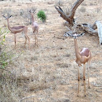
4       H. Debbi

     Finally, both Grad-CAM and CexCNN can be used for Weakly Supervised Object
Localization (WSOL), since they provide attention maps representing the most impor-
tant regions. However, our method could give better results in this regard, since it can
be easily extended to localize less important features, thus, resulting in identifying the
entire object, not only its important features.
     Causal Explanation of CNNs: The causal-based explanation methods suggest to
rely on the cause-effect principle. By employing either statistical, intervention or coun-
terfactual approaches, many causal explanation methods have been proposed in order to
give causal interpretation for CNNs decisions, or abstract the CNN models into causal
models.
     Harradon et al. [15] have considered building a causal model for CNNs, which is
a casual Bayesian model built based on extracting salient concepts. These concepts
represent then the variables in the Bayesian model. Based on the definition of causal
interventions, Narendra et al. [25] proposed structural causal models (SEM) as an ab-
straction of CNNs. This method is based on considering filters as causes, and then rank-
ing them by their counterfactual influence with respect to each convolution layer. Given
the SEM, the user would be able to get an answer for the following query or question:
what is the impact of the n-th filter on the m-th layer on the model’s predictions?”. The
main drawback of this approach is the size of the causal model generated, which could
consist of thousands of nodes and edges.
     Our approach to causality differs to previous methods in different ways. While these
methods attempt to build an equivalent causal model that acts as an explanatory model
for CNNs, our approach learns only the most important features, thus enabling class
discrimination through estimating the responsibility of each causal filter in the last con-
volution layer, where the rest of non-causal filters are omitted. From another side, our
work employs counterfactual reasoning, which comes at the top of the causal hierarchy,
in contrast to [15] and [28], which employ interventions, and association respectively.
Only [25] adopted counterfactuals similarly to our work, however, with major differ-
ences. First, with respect to counterfactual adoption, they measure the importance of
filters in term of variance, not as we do here, in term of responsibility, which repre-
sents the quantitative extension of counterfactual causality. Besides, we adopt here in
addition to responsibility, blame and causal abstraction, which make CexCNN a robust
causal framework. With respect to the use of causality for explaining CNNS, [25] does
not aim to identify salient regions, but rather, it helps to understand the inner working
of CNNs.

3   Causal explanation of CNNs

Gradient-based methods of explanation such as CAM [35] and Grad–CAM [29] are
very useful explanation methods for CNNs. However, they only explain the output ac-
tivations of a specific class in terms of the input activations, thus they are dependent
on gradients with the absence of any causal interpretation. In this section we will show
that CNNs have actually a causal structure, where the final decision at the final layer has
causal dependencies on all the previous layers. So, what we are about to do, is to show
how causality can be interpreted in CNNs, and how to define it in terms of the definition
Causal Explanation of Convolutional Neural Networks        5

of causality by Halpern and Pearl. Moreover, we will show how we can benefit from its
quantitative measures responsibility and blame to give robust explanations for CNNs
decisions.
    It is well known that the most important layers of CNNs models are the convolution
layers, which include the filters. A filter actually represents the basic element of the
network that gives activations for different regions in the image. In this section, we
will show that addressing causality in CNNs should be built upon filters. Although
some works that investigated causality on CNNs through couterfactuals addressed the
perturbation of the input image [15], we will show that in our technique, we let both the
input image as well as the network intact, without any modification and retraining.

3.1   Filters as actual causes
In this section we will show how we can define a probabilistic causal model [13] for
CNNs. Each input image consists of a specific number of pixels. In CNNs, we move
filters of specific sizes on sets of pixels, and the values obtained refer to match proba-
bilities of these filters on every region in the input image. Then, these values serve as
inputs for the flowing convolution layers. Filters with higher matches on the image’s
regions (or convoluted images in next layers) give higher activations, which will help
to decide on the final class in the last layer. So, if we think of the nature of filters in
terms of causality with respect to a CNN architecture, we find that filters represent ac-
tual causes, since their match on input image regions give rise to the activations that
lead to the final decision.
     With respect to the definition of causality by Halpern and Pearl, the actual cause X
is defined on a context. So, we need to reason on contexts in CNNs. Actually, given an
input/convolved image, we have different contexts, which represent the different regions
of the image on which we apply these filters. After defining a context u, we can also
reason on the probability function of the context P r(u), which refers to the probability
of the filter’s match given a context u. So we can say that a filter at a specific layer
fl is a cause in a region u with a probability P rfl (u) for such a decision, where the
filters probabilities can be returned based on the activations of the feature maps of the
last convolutional layer. Now the remaining task is to define ϕ in CNNs, what would
ϕ represent? It is evident that ϕ would represent the final class identified by a CNN,
for instance a hummingbird (see Fig. 1). However, with CNNs, the class predicted is
returned with a probability, thus ϕ should not be just a Boolean formula that refers to
the class predicted being a hummingbird, but rather is returned with a probability P .
     We should recall that an actual cause is defined based on counterfactual theory.
Formally, let us denote by F the set of all filters. Now we can introduce the definition
of an actual cause in CNNs.
Definition 1. Actual cause let us consider a filter at a specific layer l denoted fl ∈ F .
We say that fl is an actual cause for a decision ϕ, if its own removal, where all the
filters are kept the same, decreases the prediction probability P of ϕ by p.
                                                             ϕ
    The set of filters F can be partitioned into two sets FW    and FZϕ , where the set FW
                                                                                         ϕ

refers to filters causing the prediction ϕ, i.e. their removal will decrease the prediction
probability P , whereas FZϕ are not causal, in way that removal of a filter in FZϕ does not
6 H. Debbi
affect P , or increases it. When the removal of a filter leads to increasing P , this means
that this filter has a negative effect on the decision, which means that it is responsi-
ble for increasing the prediction probability of another class, not the current class (see
Fig. 1). With this definition in hand, we can now introduce the definition of a filter’s
responsibility.
Definition 2. Responsibility The degree of responsibility of a filter fl for a prediction
ϕ denoted dr(fl , ϕ) is 0 if fl ∈ FZϕ , i.e. fl is not a cause, and otherwise is 1/(|fW |+1),
ϕ ϕ
where fW ⊆ FW refers to the minimal subset such that their removal FW − fW makes
decreasing the probability P below Pt counterfactually depends on fl , where Pt refers
to a probability threshold.
So the filter’s importance for such a prediction is measured with regard to its re-
sponsibility, where the most responsible filter would be the one whose removal results
in decreasing P significantly. A most responsible filter would have 1 as a degree of
responsibility, i.e. |fW | = 0, if its own removal decreases P below the probability
threshold Pt .
W1 Counterfactual,
FIlter1 Hummingbird question:What would
W2
with P=0.90 the probability of
… … hummingbird , if one
FIlter2 … …
.. of these filters is
..
… Wn
..
.
Output channels removed :
Filter n
Input image Convolution Layers Last Convolution Layer Predictions
Filter1 is causal, since
W1 its removal decreases
FIlter1
Hummingbird P by p=0.04
W2
with P=0.85
FIlter2 … …
… …
..
..
… Wn
..
.
Filter n
Filter2 is causal, and
W1
could have more
FIlter1 Hummingbird
W2 responsibility than
with P=0.82
Filter1
FIlter2 … …
… Wn …
..
..
…
..
.
Filter n
W1
FIlter1 Hummingbird Filter n is not causal,
W2 since its removal
with P=0.95
increases P
FIlter2 … …
… Wn …
..
..
…
..
.
Filter n
Filters
Probabilities Filters
Responsbilities
{
The most important
features to blame
Fig. 1: CexCNN architecture: Localizing the most discriminative regions to blame,
which is performed by projecting back the product of filters responsibilities and their
activations. Based on causality abstraction, only the last convolution layer is considered
for this computation.
The definitions of actual cause and responsibility are very useful for getting an in-
sight on how CNN decisions were derived, thus they could be mainly useful for model
diagnosis. However, for the main purpose of this paper, which is providing interpretable
Causal Explanation of Convolutional Neural Networks          7

explanations of CNNs decisions, these definitions are not sufficient. In order for the ex-
planation to be interpretable, it should highlight the features or regions of interest in the
input image. Here comes the definition of blame, which can be used to localize the sets
of pixels in the input image that should be blamed the most for the decision ϕ. Once we
answer this question, the explanations can be given to the user by highlighting discrimi-
native regions. So, the remaining task is to relate the definition of filters responsibilities
to regions blame.

Definition 3. Blame Let us denote by K the set of regions in an input image. The degree
of blame for a region σ ∈ K for a prediction ϕ denoted db(σ, ϕ) is
                                         X
                        db(σ, ϕ) =                  dr(fl , ϕ)P rfl (σ)                   (1)
                                          ϕ
                                     fl ∈FW ,σinK

     So the degree of blame db for a region σ is computed as the sum of the products
of every causal filter match’s probability in this region with its responsibility. In other
words, the regions that should be blamed the most for a decision ϕ, would be the ones
having the highest match probabilities with the most responsible filters. Those regions
are identified critical for the decision ϕ, and when returned together they show inter-
pretable features on the input image.
     Abstraction of causality
     Beckers and Halpern [5] investigated the problem of abstracting causal models,
when micro variables have causal effect on macro variables at higher levels. This in-
tuition behind abstraction of causal models leads us to consider for explaining such a
decision, only the filters of the last convolution layer, since they represent the top macro-
variables. We will show that they will be sufficient to estimate the degree of blame for
every region in the input image.
     What we aim to do through explanation is to identify at the final layer which impor-
tant features led to such a decision. For instance, forehead and tail in the input image
have led to the decision of a hummingbird (see Fig. 1). In other words, which features
should be blamed for such a decision.
     The importance of an image’s regions are identified by projecting back the products
of the activations of the last convolutional feature maps that refer to filters match prob-
abilities and the responsibilities associated with these filters. In other words, among all
outputs of the last convolution layer, we project back only the output of filters with high
responsibilities. Similar to CAM, CexCNN provides heatmaps as grids of scores.

4   Experiments

In this section we test our method CexCNN on many datasets and architectures. We first
conduct an experiment on two different architectures: VGG16 and Inception trained
on the same dataset: ImageNet [9]. Then we test it on a third architecture, which is
LeNet[18] trained on MNIST [19]. These experiments would show the effectiveness of
CexCNN despite the architecture and the dataset in use. One common thing is that none
of these architectures needs to be modified or retrained.
8      H. Debbi

              (a) Image          (b) CexCNN          (c) Grad-CAM

                   (d)              (e)                  (f)

                  (g)                (h)                  (i)

                  (j)                (k)                  (l)

                  (m)                (n)                  (o)

                  (p)                (q)                  (r)

                  (s)                 (t)                 (u)

Fig. 2: Discriminative image regions returned by CexCNN compared to Grad-CAM.
The images are from ImageNet ILSVRC [27], on which VGG16 is trained. The
heatmaps generated by CexCNN refer to the most important features to blame.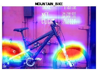
Causal Explanation of Convolutional Neural Networks           9

     All the experiments are mainly based on measuring the responsibility of each filter
of the last convolution layer. To do so, we have to perform removing or zeroing each
filter in order to measure its effect. In the literature there exist some libraries for pruning
CNNs through removing specific filters [2,21].

4.1   Evaluating Visualizations

Since we introduce CexCNN as an explanation technique, we choose to evaluate it
against some desirable properties that every explanation method for ML models should
meet. Some properties are summarized in [24].
    In this experiment we first test our method on VGG16 trained on the ImageNet
dataset [9]. We choose the last convolution layer of the model to be the top of the causal
hierarchy. This layer includes 512 filters, among them we consider only the most re-
sponsible ones. Filters whose removing has no effect on the predicted class probability,
or has a positive effect, are not causes, and thus they are not considered for computing
responsibility and blame. For the rest of causal filters, we compute their responsibilities,
and then project their values on the original image through all the previous layers, in
order to obtain the blame of each region. The most blamed regions in the image would
have the highest heatmaps.
    Examples of some classes and the heatmaps generated by CexCNN are depicted in
Fig. 2. The explanations provided by our method are compared to those provided by
Grad-CAM in the same figure.
    Comparing to Grad-CAM, we find that our method sometimes localizes nearly the
same important features that Grad-CAM localizes, like umbrella, and sometimes it lo-
calizes different features. For instance, with boxer, our method detects the face as the
most important feature(k), however with Grad-CAM, the chest is considered more im-
portant (l).
    A) Discriminative ability We see that CexCNN localizes important features that
should be blamed the most. Besides, it is highly sensitive, where critical regions are
clearly visualized, without highlighting regions on the other objects. For instance, the
boxer with a hat (e), the hat is not highlighted. In the second image of boxer (h), the belt
is excluded as well. Other examples include umbrella and mountain bike, whose only
discriminative features are highlighted despite the presence of other objects.
    B) Stability
    Another important property that CexCNN satisfies is stability. This property aims
to measure how similar are the explanations for similar instances in the same model.
We see that our framework satisfies very well this property.
    If some features are considered most important for a specific class, they are consid-
ered in every instance of this class. They can be just affected by which features are in
foreground or background pixels. This can be noticed in boxer class, where the face is
most important, in addition to chest with low importance (h). In this class, please note
that compared to Grad-CAM, our method is more stable, it always focuses on the head
as the most important feature, however, Grad-CAM sometimes considers chest as the
only important feature, ignoring completely the head (i). With the same class, we notice
that in figure (f), Grad-CAM failed to localize the face feature, where it has been fooled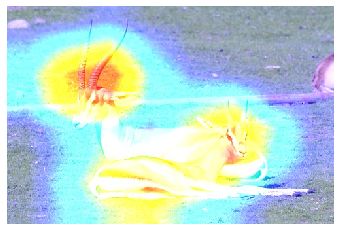
10      H. Debbi

apparently by the hat on the boxer’s head, but CexCNN is always stable by returning
the face as the most important feature in an accurate way.
    In other classes such as gazelle, it is clear that our method outperforms Grad-CAM
for localizing important features. See for instance (m), our method was able to localize
the features of all visible gazelles similarly in the input image (n). However, with Grad-
CAM, the heatmap is wrongly localized (o). Always with the same class, we see that
for the two gazelles in figure (j), our method for the two gazelles localizes the same
important features (k), whereas for Grad-CAM the features returned are not stable (l),
with much noise on the grass background.

               (a)                (b)               (c)                (d)

      Fig. 3: Explanation results by CexCNN for Inception trained on ImageNet

    C) Consistency: This property attempts to measure how does an explanation differ
between models that have been trained on the same dataset. To this end, in addition to
VGG16, we tested CexCNN on Inception trained on Imagenet as well.
    Comparing to VGG16, providing explanations for Inception is more challenging,
since Inception consists of many modules, which consist of multiple convolution layers.
The convolution layers considered by CexCNN are the last concatenated ones. While
the last convolution layer of VGG16 consists of 512 filters, the last convolution layers
of Inception when concatenated consist of 2048 filters. Similar to VGG16, we have
to measure the responsibility of each filter and use this information to find the most
important features to blame.
    Before presenting the results of this experiment, we should note here that providing
similar explanations for different models on the same instances is only possible if the
two models see the world similarly, i.e. if the models focus on the same features to
make a decision. Actually, providing explanations could be itself useful for identifying
if different models see the world in a similar way. However, in order to evaluate con-
sistency, it is necessary for the explanations to be stable with respect to each model.
The results of stable explanations provided by CexCNN on Inception for some classes
compared to those returned by VGG16 are presented in Fig. 3. We see that for some
instances such as umbrella and boxer, the explanations are very similar, which means
that both VGG16 and Inception focus on the same features for predicting these classes.
However, with other classes such as mountain bike, Inception focuses on a different
important feature, which absolutely discriminates mountain bike as well from other
classes.
    D) Robustness against Adversarial Attacks Goodfellow et al.[11] have discov-
ered a critical weakness for DNNs models, which is adversarial examples or adversarial
attacks. Goodfellow et al. showed that perturbating input images through introducing
Causal Explanation of Convolutional Neural Networks 11
noise to the original images, in way that they look identical to the human eye, such
perturbation could fool the network to completely misclassify the input image. In this
section, we will show how CexCNN performs against perturbed images that have been
misclassified by VGG16. For generating perturbations we use the FGSM method [11].
Some qualitative examples are presented in Fig. 4. As we see, although CexCNN is
affected slightly by the perturbations, it always try to focus on the same discriminative
regions.
Fig. 4: Robustness against adversarial attacks:heatmaps returned by CexCNN
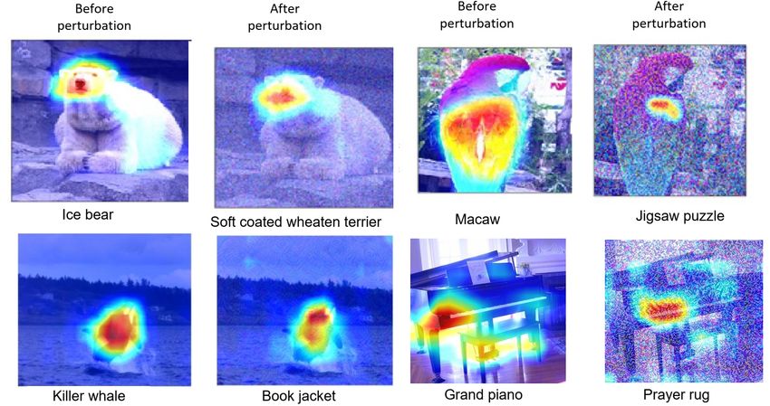
4.2 MNIST
We tested our method on LeNet architecture trained on MNIST dataset [19]. We con-
sider the last layer of the LeNet architecture with 64 filters. In this experiment we tried
another strategy for computing counterfactual information and measuring responsibility
and blame. Since this dataset is small (10 classes), with simple classes (digits), not com-
plex ones comparing ImageNet, we measured the causal effect on the accuracy of the
entire model, not just the prediction probability of an individual class. The heatmaps as
generated by our method on every digit compared to heatmaps generated by Grad-CAM
are presented in Fig. 5. These results are obtained using the Keras-vis tool [3].
We see that our method clearly outperforms the important regions localized by
Grad-CAM. The quality of the explanations generated is clearly better than Grad-CAM,
because for every digit it is sufficient to decide on the input image just by considering
the highlighted features related to this digit. For some digits, 9 for instance, Grad-CAM
fails to generate explanations at all. Another important thing about the effectiveness
of our method compared to Grad-CAM, is that our method returns stable explanations
despite the modifier in use.
4.3 Weakly Supervised Object Localization (WSOL)
WSOL has been recently addressed by many researchers for different visual tasks
[35,31,7]. WSOL aims to localize objects with only image-level labels, under a gen-
eral assumption that only one object of the specific category is present in the input12 H. Debbi
Fig. 5: CexCNN results on MNIST compared to Grad-CAM
image. One main drawback of existing WSOL methods such as CAM, which gave a
rise to other WSOL methods, is that it localizes only the most discriminative features
of an object rather than all the features, which leads logically to a less performance in
object localization task. Kumar and Lee [31] for instance tried to tackle this issue by
modifying the input image by randomly removing grid patches, thus forcing the net-
work to be meticulous for WSOL, by identifying all the object’s features not only the
most discriminative ones. In this section, we will show that CexCNN provides good
results in this regard. To make CexCNN good in WSOL, we should consider all the
ϕ
causal filters FW , not just the most responsible ones. This results in identifying all the
object’s parts from the most discriminative (having the highest blame dB) to parts with
low discrimination (having the lowest blame dB). To show the effectiveness of Cex-
CNN for WSOL, we provide qualitative (See Figure 6) as well as quantitative results
(See Table 1) on the ILSVRC validation dataset, which consists of 50.000 images of
1000 categories. The results are compared to CAM. We see in Figure 6 that CexCNNCausal Explanation of Convolutional Neural Networks 13
localizes in a better way the concerned object, since it could look on all its features,
from the most important to the less important ones, whereas CAM is designed to focus
only on the most discriminative regions. Both CexCNN and CAM are evaluated in the
same setting, on VGG16 without any architectural modifications.
Heatmap Bounding box Bounding box Heatmap Bounding box
(CexCNN) (CexCNN) (CexCNN) (CAM) (CAM)
Fig. 6: Qualitative object localization results
Method GT-known Loc
CAM 31.71
CexCNN 67.65
Table 1: Quantitative object localization results for CexCNN compared to CAM on
VGG16
For quantitative evaluation, a set of evaluation metrics are commonly used to access
the performance of WSOL methods. These metrics are Top-1/Top-5 localization accu-
racy and localization accuracy with known ground truth class (GTKnown Loc). While
Top-1/Top-5 represent both the classification and localization, GT-Known Loc is true14 H. Debbi
for an input image if given the ground truth class, the intersection over union (IoU)
between the ground truth bounding box and the predicted box is at least 50%. Since we
are interested here in evaluating CexCNN only for object localization, not for classifi-
cation, we decided to consider only GTKnown Loc. Besides, Choe et al. [7] have shown
in their evaluative study of existing WSOL methods that Top-1/Top-5 localization might
be misleading, and thus they suggest to consider the GT-known metric. The experiments
are conducted by performing a small modification on the dataset by ignoring the im-
ages having multiple bounding boxes. The reason is that close multiple instances of the
target class result in overlapped heatmaps, which could be misleading[7]. The resulted
dataset consists of 38.285 images. The localization results of CexCNN compared to
CAM are provided in Table 1. Both CexCNN and CAM were executed on the same
dataset. We see that CexCNN clearly outperforms CAM in WSOL. Moreover, based on
the reproduced results in [7] for evaluating existing WSOL methods, with 67.65 accu-
racy, CexCNN outperforms all the existing methods that have been evaluated on VGG
with global average pooling (VGG-GAP), where the best WSOL accuracy reported was
62.2.
4.4 Fine-tuning parameters and compact representation
Network pruning aims to compress CNN models in order to reduce the network com-
plexity and over-fitting. This requires pruning and compressing the weights of various
layers without affecting the accuracy of these models. Some previous works on fine-
tuning CNNs aimed at computing some metrics for every filter in order to generate a
compact network [21]. Li et al.[21] showed that pruning filters of multiple layers at once
can be useful and gives a good view on the robustness of the network. In this regard, we
may consider the filter’s responsibility as a useful metric for this purpose. We conduct
experiments on LeNet trained on MNIST. The experiments are based on removing the
filters with low responsibilities at each layer, and then calculate the impact of their re-
moval on the model’s accuracy. The results presented focus on the number of the filters
pruned and the number of network’s parameters reduced, by allowing the accuracy to
be very close to the original one. While pruning without retraining might be harmful
for the model accuracy [21,14], we will show that our results are good enough without
retraining.
LeNet consists of two convolution layers: the first consists of 20 filters, and the last
one consists of 50 filters. For LeNet on MNIST, the best results in terms of accuracy
are obtained by removing (2/20) filters (10%) of the first convolution layer, and (12/50)
filters (24%) of the last one. This operation results in reducing the network’s parameters
from 639.760 (original model) to 486, 884 (23.90%), and resulting in a good accuracy,
which has been reduced just from 0.9933 to 0.9928 (See Table 2).
We notice that conv1 is more sensible for filters pruning, thus we want to chal-
lenge our technique on accuracy against the number of reduced parameters by consid-
ering only conv2. The results are presented in the same table. While most of pruning
techniques consider retraining the model, Han et al.[14] have analyzed in addition the
trade-off between accuracy and number of parameters without retraining. The results
as described here are very close to the ones reported in [14]. We see that we are able toCausal Explanation of Convolutional Neural Networks 15
Parameters Filters pruned conv1 Filters pruned conv2 total pruned Pruned parameters % Error%
639.760 2/20 12/50 14/70(20%) 152.876(23.90%) 0.05
639.760 13/20 28/50 41/70(58%) 355.068(55.92%) 5.1
639.760 0/20 36/50 36/70(51.42%) 456.516(71.35%) 3.03
639.760 0/20 39/50 39/70(55.71%) 494.559(77.30%) 4.5
Table 2: Results after pruning less responsible filters for LeNet trained on MNIST
reduce the number of parameters by 77.30% , which results in dropping the accuracy
from 0.9933 to 0.9483.
5 Conclusion and Future Work
In this paper we provided CexCNN, a causal explanation technique for CNNs. CexCNN
employs the theory of causality by Halpern and Pearl, in addition to their quantitative
measures: responsibility and blame, as well as causality abstraction. We showed that
weighting filters by their responsibilities and then projecting this information back in
the input image, allows the localization of the most important features to blame for such
a decision.
We evaluated CexCNN on many datasets and architectures and it has shown good
results given a set of evaluation properties for explanation methods. Although the main
concern is to localize the most discriminative regions, we showed that CexCNN outper-
forms Grad-CAM and known existing methods for WSOL. In addition, we showed that
CexCNN could stand as a good pruning technique.
As future work, we aim to address the usefulness of CexCNN for defending against
adversarial attacks, as well as its application in transfer learning.
References
1. Investigate. https://github.com/albermax/innvestigate 3
2. keras-surgeon. https://github.com/BenWhetton/keras-surgeon 9
3. Keras visualization toolkit. https://github.com/raghakot/keras-vis 11
4. Avanti, S., Peyton, G., Anshul, K.: Learning important features through propagating activa-
tion differences. p. 3145–3153. ICML’17 (2017) 3
5. Beckers, S., Halpern, J.Y.: Abstracting Causal Models. In: AAAI (2017) 2, 7
6. Chockler, H., Halpern, J.Y.: Responsibility and blame: A structural-model approach. J. Artif.
Int. Res. 22(1), 93–115 (2004) 2
7. Choe, J., Oh, S.J., Lee, S., Chun, S., Akata, Z., Shim, H.: Evaluating weakly supervised
object localization methods right. In: CVPR. pp. 3130–3139 (2020) 11, 14
8. D. Gordon, A. Kembhavi, M.R.J.R.D.F., Farhadi, A.: Iqa: Visual question answering in in-
teractive environments. In: In arXiv:1712.03316 (2017) 1
9. Deng, J., Dong, W., Socher, R., Li, L., Kai Li, Li Fei-Fei: Imagenet: A large-scale hierarchi-
cal image database. In: CVPR. pp. 248–255 (2009) 7, 9
10. Girshick, R., Donahue, J., Darrell, T., Malik, J.: Rich feature hierarchies for accurate object
detection and semantic segmentation. In: CVPR. pp. 580–587 (2014) 116 H. Debbi
11. Goodfellow, I.J., Shlens, J., Szegedy, C.: Explaining and harnessing adversarial examples.
In: ICLR (2015) 10, 11
12. Halpern, J., Pearl, J.: Causes and explanations: A structural-model approach part i: Causes.
In: Proceedings of the 17th UAI. pp. 194–202 (2001) 1, 2
13. Halpern, J.Y., Pearl, J.: Causes and explanations: A structural-model approach. part ii: Ex-
planations. British Journal for the Philosophy of Science 56(4), 889–911 (2008) 2, 5
14. Han, S., Pool, J., Tran, J., Dally, W.J.: Learning both weights and connections for efficient
neural networks. In: NIPS (2015) 14
15. Harradon, M., Druce, J., Ruttenberg, B.E.: Causal learning and explanation of deep neural
networks via autoencoded activations. In: CoRR abs/1802.00541 (2018) 1, 4, 5
16. Krizhevsky, A., Sutskever, I., Hinton, G.E.: Imagenet classification with deep convolutional
neural networks. Commun. ACM 60(6), 84–90 (2017) 1
17. Lecun, Y., Bottou, L., Bengio, Y., Haffner, P.: Gradient-based learning applied to document
recognition. Proceedings of the IEEE 86(11), 2278–2324 (1998) 1
18. Lecun, Y., Bottou, L., Bengio, Y., Haffner, P.: Gradient-based learning applied to document
recognition. Proceedings of the IEEE 86(11), 2278–2324 (1998) 7
19. LeCun, Y., Cortes, C., Burges, C.: Mnist handwritten digit database. ATT Labs [Online].
Available: http://yann.lecun.com/exdb/mnist 2 (2010) 7, 11
20. Lewis, D.: Causation. Journal of Philosophy 70, 556–567 (1972) 2
21. Li, H., Kadav, A., Durdanovic, I., Samety, H.: Pruning filters for efficient convnets. In: ICLR
2017. pp. 1–13 (2017) 9, 14
22. Long, J., Shelhamer, E., Darrell, T.: Fully convolutional networks for semantic segmentation.
In: CVPR. pp. 3431–3440 (2015) 1
23. Lundberg, S.M., Lee, S.I.: A unified approach to interpreting model predictions. In: NIPS. p.
4768–4777 (2017) 3
24. Molnar, C.: Interpretable Machine Learning A Guide for Making Black Box Models Explain-
able (2018), https://christophm.github.io/interpretable-ml-book/ 9
25. Narendra, T., Sankaran, A., Vijaykeerthy, D., Mani, S.: Explaining deep learning models
using causal inference. In: arXiv:1811.04376 (2018) 4
26. Ribeiro, M.T., Singh, S., Guestrin, C.: ”why should i trust you?”: Explaining the predictions
of any classifier. p. 1135–1144. KDD ’16 (2016) 3
27. Russakovsky, O., Deng, J., Su, H., Krause, J., Satheesh, S., Ma, S., Huang, Z., Karpathy, A.,
Khosla, A., Bernstein, M., Berg, A.C., Fei-Fei, L.: Imagenet large scale visual recognition
challenge. Int. J. Comput. Vision 115(3), 211–252 (2015) 8
28. Schwab, P., Karlen, W.: Cxplain: Causal explanations for model interpretation under uncer-
tainty. NeurIPS pp. 10220–10230 (2019) 1, 4
29. Selvaraju, R.R., Cogswell, M., Das, A., Vedantam, R., Parikh, D., Batra, D.: Grad-cam: Vi-
sual explanations from deep networks via gradient-based localization. In: ICCV. pp. 618–626
(2017) 3, 4
30. Simonyan, K., Vedaldi, A., Zisserman, A.: Deep inside convolutional networks: visualising
image classification models and saliency maps. In: In arXiv:1312.6034 (2013) 1
31. Singh, K.K., Lee, Y.J.: Forcing a network to be meticulous for weakly-supervised object and
action localization. In: CVPR (2017) 11, 12
32. Smilkov, D., Thorat, N., Kim, B., Viegas, F.B., Wattenberg, M.: Smoothgrad: removing noise
by adding noise. In: CoRR, vol. abs/1706.03825 (2017) 3
33. Sundararajan, M., Taly, A., Yan, Q.: Axiomatic attribution for deep networks. In: ICML. p.
3319–3328 (2017) 3
34. Zeiler, M., Fergus, R.: Visualizing and understanding convolutional networks. In: Computer
Vision – ECCV 2014. vol. LNCS, pp. 818–833 (2018) 1
35. Zhou, B., Khosla, A., Lapedriza, A., Oliva, A., Torralba, A.: Learning deep features for
discriminative localization. In: CVPR. pp. 2921–2929 (2016) 3, 4, 11You can also read