CRYPTO PROXIMA AN ANALYSIS OF AUTONOMOUS BITCOIN TRADING SIMON ANDERSSON JAKOB HÄGGSTRÖM URLICH ICIMPAYE HJALMAR LINDSTEDT - DIVA
←
→
Page content transcription
If your browser does not render page correctly, please read the page content below
MAT-VET-F-21012

                               Examensarbete 15 hp
                                         Juni 2021

Crypto Proxima
An analysis of autonomous Bitcoin trading

Simon Andersson
Jakob Häggström
Urlich Icimpaye
Hjalmar Lindstedt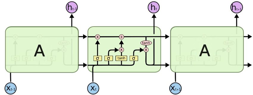
Abstract
                                      Crypto Proxima

                                      Simon Andersson, Jakob Häggström, Urlich Icimpaye, Hjalmar Lindstedt

Teknisk- naturvetenskaplig fakultet
UTH-enheten                           The purpose of this project is to analyze to what extent it is
                                      possible to profit from autonomous bitcoin (BTC) trading. This was
Besöksadress:                         tested by using three different models in varying complexity and
Ångströmlaboratoriet
Lägerhyddsvägen 1                     simulating these using real market data. The tested models were a
Hus 4, Plan 0                         Long Short Term Memory (LSTM) neural network, a technical analysis
                                      model based on moving averages (MA), and a random model that
Postadress:                           generates different buy and sell points. The LSTM model showed
Box 536
751 21 Uppsala                        indications of possible profitability when trading at higher
                                      frequencies. For certain parameters, the model outperformed the
Telefon:                              market. The MA model was tested using a combination of different
018 – 471 30 03                       parameters for a total of 48 simulations. These had different trade
Telefax:                              offs based on the combinations, where some were able to predict the
018 – 471 30 00                       market to some extent. Regarding the random interval model, the
                                      results showed that the simulations were normally distributed around
Hemsida:                              approximately half of the market gain or loss. The reason behind this
http://www.teknat.uu.se/student
                                      is likely because the model is invested half of the time, and idle
                                      the other half. It seems that autonomous trading definitely can be
                                      profitable, however choosing the optimal parameters remains as a
                                      subject for further research.

                                      Handledare: Kaj Nyström
                                      Ämnesgranskare: Natalia Ferraz
                                      Examinator: Martin Sjödin
                                      ISSN: 1401-5757, MAT-VET-F-21012
                                      Tryckt av: Uppsala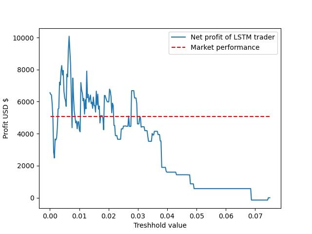
Populärvetenskaplig sammanfattning
    I följande projekt har det undersöks i vilken utsträckning det är
möjligt att dra till nytta av autonom bitcoin-handel (BTC). Detta
testades genom att använda tre olika modeller av varierande kom-
plexitet och simulera dessa med marknadsdata. De modellerna som
prövades var ett neuralt nätverk som kallas ”Long Short Term Mem-
ory” (LSTM), en teknisk analysmodell baserad på glidande medelvärden
(MA) och en slumpmässig modell som slumpmässigt genererar olika
köp- och säljsignaler. LSTM-modellen visade indikationer på möjlig
lönsamhet vid handel på högre frekvenser. För vissa parametrar överträffade
modellen marknaden. MA-modellen testades med en kombination av
olika parametrar för totalt 48 simuleringar. Dessa hade olika avvägningar
baserat på kombinationerna, där vissa kunde förutsäga marknaden i
viss utsträckning. När det gäller den slumpmässiga modellen visade
resultaten att simuleringarna normalt fördelades runt ungefär hälften
av marknadsvinst- eller förlusten. Anledningen till detta beror troli-
gen på att modellen var investerad hälften av tiden och inaktiv den
andra hälften. Autonom handel kan vara lönsam, men att välja de
optimala parametrarna förblir emellertid ett ämne för vidare forskn-
ing.
Contents
1 Introduction 1
1.1 Background . . . . . . . . . . . . . . . . . . . . . . . . . . . . 1
1.2 Purpose . . . . . . . . . . . . . . . . . . . . . . . . . . . . . . 1
2 Theory 2
2.1 Long Short Term Memory . . . . . . . . . . . . . . . . . . . . 2
2.2 Moving Average . . . . . . . . . . . . . . . . . . . . . . . . . . 4
2.3 Random Time Intervals . . . . . . . . . . . . . . . . . . . . . . 5
3 Method 6
3.1 Data preprocessing . . . . . . . . . . . . . . . . . . . . . . . . 6
3.1.1 API . . . . . . . . . . . . . . . . . . . . . . . . . . . . 6
3.1.2 TimeSeries . . . . . . . . . . . . . . . . . . . . . . . . . 6
3.2 Model Implementation . . . . . . . . . . . . . . . . . . . . . . 7
3.2.1 LSTM . . . . . . . . . . . . . . . . . . . . . . . . . . . 7
3.2.2 Moving Average . . . . . . . . . . . . . . . . . . . . . . 9
3.2.3 Random Intervals . . . . . . . . . . . . . . . . . . . . . 9
3.2.4 Simulation . . . . . . . . . . . . . . . . . . . . . . . . . 9
4 Results 10
4.1 LSTM . . . . . . . . . . . . . . . . . . . . . . . . . . . . . . . 10
4.2 Moving Average . . . . . . . . . . . . . . . . . . . . . . . . . . 12
4.3 Random Intervals . . . . . . . . . . . . . . . . . . . . . . . . . 14
5 Discussion 16
5.1 LSTM . . . . . . . . . . . . . . . . . . . . . . . . . . . . . . . 16
5.2 Moving average . . . . . . . . . . . . . . . . . . . . . . . . . . 17
5.3 Random intervals . . . . . . . . . . . . . . . . . . . . . . . . . 18
6 Conclusion 181 Introduction
1.1 Background
Ever since the first stock market opened in Amsterdam 1653 people have
been trying to predict the future prices of goods and assets [1]. Regardless of
various bursted bubbles and financial crises, the stock market has survived.
The recent invention of cryptocurrencies have allowed for a new type of mar-
kets where these cryptocurrencies are traded. These exchanges work in the
same manner as a regular stock exchange, with a few exceptions. The stock
market is only open for a few hours on working days, while the cryptocur-
rency exchanges are open everyday around the clock.
One advantage that cryptocurrencies provide is that they are available to
anyone in the entire world. While you might only be able to buy stocks in
your own country and a few others, these purchases must be done within the
legislation of the laws and bureaucratic systems in that particular country
and stock exchange. This is in direct contrast to cryptocurrencies where any-
one, anywhere, can buy cryptocurrency. Since it is a decentralized currency,
nobody can legislate the terms of conditions. This also allows anyone to send
crypto to anyone else in the world without having any obstacles or having to
use an intermediator[2][3].
Another key difference between stock- and cryptoexchanges is that cryp-
tocurrencies are also a means of payment. However, it is not yet advanta-
geous to use these cryptocurrencies over regular fiat currencies when trading
goods online. This is why BTC is often treated as an asset, or store of
value, instead of an actual currency. Since the value of BTC is significantly
higher (in relation to other fiat currencies) and extremely volatile, it makes
it unreliable and inconvenient to use as a means of payment in practise [3].
1.2 Purpose
In this project the goal is to examine what type of methods is suitable to use
in order to autonomously trade BTC and to maximize the profit. Three dif-
ferent methods were used, and were tested using different hyperparameters.
Based on simulations they were compared on the profit that they made, us-
ing data from the BTC market. The selected models had varying complexity
1in order to see if this had any impact on the profitability. These methods
are not exclusively used to analyze data from BTC, they could be used to
analyze any data from a time series. The main reason for why BTC was
chosen to be analyzed in this project is due to the availability of data.
2 Theory
2.1 Long Short Term Memory
The importance of order and causality is recurrent in various fields. A simple
example is predicting the last word of a sentence. You need the permutation
of the earlier words in order to understand the context of the sentence, which
gives the basis of a valid prediction. Another problem that takes order into
account, is this very project. The aim is to predict future prices, and to
do so you need to take past data in time into account in order to make a
valid prediction. A model that might be a appropriate fit to this problem,
is a Long Short Term Memory network. LSTM (Long Short Term Memory)
networks is a type of recurrent neural network that has the ability to store
important information from the past [4]. It deciphers patterns in a text or
a time series by processing information trough a network of hidden cells, or
also called hidden units, which has the architecture as shown in figure 1.
Figure 1: The architecture of a LSTM network. Taken from [4]
Each cell that is shown in figure 1 is built in different gates that decides
whether to forget or to remember current and past information by using
sigmoid and hyperbolic tangents as acivation functions. The information is
stored in in a so called cell state Ct , which is the essential building stone in a
2LSTM network. Every hidden unit has its own cell state, but not necessarily
unique, since it is connected with the neighbouring cell of the last timestep.
If the gates decide to keep the cell state of the past and neglect the infor-
mation from the current timestep, then the cell last state flows through the
current hidden unit unchanged.
How does the LSTM network operate? Firstly, the information from the
input xt , which is often a tensor of dimension (number of sequences, length
of each sequence, number of features in each sequence), is concatenated with
output of the last cell ht−1 . Thereafter, the new tensor flows into the first
layer, which is the forget gate. Here it is decided if the output of the last
cell is still relevant in respect to the current input. For example, if you are
to predict the next price of BTC, and the sequence at the earlier timestep
indicates stagnation but the current sequence implies an increase, then it is
not necessary to keep the information from the past. In a LSTM point of
view, the concatenated tensor goes through a sigmoid activation function,
which transforms all values into the range zero to one, where zero means
forget entirely and one remember everything.
After deciding if the information of the past is worth keeping, you also need
to evaluate the relevance of the new information. This is done when the
information tensor enters the input gate layer. The gate has two operations
that work in parallel on the information tensor. Firstly you decide on what
extent you are to remember the new information. This is done in similar
fashion to the forget gate where the tensor flows into a sigmoid function that
decides the relevance of the current information. The input gate layer also
calculates a candidate C̃t for the current cell state by using a hyperbolic tan-
gent function with the input tensor as input. Finally, the current cell state
becomes the sum of the old and new candidate weighted with the output of
the corresponding sigmoid function of its gate. In mathematical terms:
Ct = ff orget ∗ Ct−1 + finput ∗ C̃t (1)
The last part of the cell is the output gate. The output from this gate is
mostly decided by the current cell state, where the gate is simply a hyperbolic
tangent function the cell state as input multiplied with a sigmoid function,
in similar manner to the other gates. In order to interpret the output from
the LSTM network, you need to connect a dense layer to the output layer.
The choice of dense layer depends on the application, for instance, if you are
3to predict the next word in a sentence, then a dense layer with a softmax
function that calculates the next word with a certain probability would be a
appropriate choice [5].
2.2 Moving Average
Another model used in the project was the moving average model, MA. It
utilises three parameters of a time series to make decisions such as buy and
sell.
• LA - The long average,
• SA - The short average
• ∆ - The band width
LA is an arithmetic average of the price calculated over a given time pe-
riod. SA is also an arithmetic average, calculated over a smaller time period
than the long average. The reason why it’s called a moving average is because
these averages are updated along the data set. SA could be calculated for
the latest hour, and when given new price data it’s calculated again. Finally,
∆ is a constant which defines a band region B together with LA. This region
is defined as LA ± ∆.
At every time instance, SA is compared against B, (the sum or difference
of LA and ∆). A sell signal would happen if SA is larger than the sum of
∆ and LA, given that there is an asset to sell. On the other hand, a buy
signal occurs when the short average is smaller than difference between the
long average and the lower boundary. The algorithm is as follows:
1 i f ( ( SA > LA + D e l t a ) and have a s s e t ) :
2 return ’ S e l l ’
3 e l i f ( ( SA < LA − D e l t a ) and not have a s s e t ) :
4 return ’ Buy ’
When the a sell signal occurs all of the asset are sold, while a buy signal only
occurs if there’s no asset in the portfolio. An example of how the algorithm
works can be visualised in figure 2.
4Figure 2: A visualisation of the algorithm behind MA
The short and long average are the green and red lines respectively, while
the blue line is the price and the dashed lines are the border of region B.
The green and red dots in the graph indicate when the trading bot bought
or sold its assets.
The idea behind the algorithm is that SA detects temporary price trends,
while LA represents a more stable, long term trend. When SA crosses the
lower bound of region B the asset might be undervalued, which is a buy-
signal, and vice versa for the upper bound.
2.3 Random Time Intervals
The price of BTC is highly chaotic, and very hard to predict in general.
A random model is an interesting baseline to compare the other models
against.
53 Method
3.1 Data preprocessing
3.1.1 API
Binance is a criptocurrency exchange, where investors can trade crypturren-
cies. Binance also offers an application programming interface (API). That
allows users to connect to Binance’s servers via several programming lan-
guages and pull data. Historical data on BTC was collected with features
such as opening price, high, low, closing price, volume, quote asset volume,
number of trades, taker buy price and taker buy quote asset volume. The
data gathered spanned from 2017 October to 2021 April. The time incre-
ments between each datapoint was one minute.
To achieve the aforementioned data gathering, the API was used in Python
programming language. The function ”get historical klines” was used to re-
trieve the historical data, which returned the data in array format [6]. This
was then converted to a data frame, because of the functionality it offers. The
features were normalized in order to reduce the training time, as followed:
x−µ
(2)
σ
where x is the sample, µ is the mean of the training samples and σ is the
standard deviation of the training samples. This was done using scikit-learn’s
prepossessing package [7] .
3.1.2 TimeSeries
The output from the API was csv-file. The package pandas offers many
features and functionalities when it comes to these files [8]. A new class,
TimeSeries, was defined in order to provide something more niched for our
project.
A TimeSeries class object is initialised with a csv-file or pandas DataFrame
from the API. The class extracts the properties of interest from the data,
and saves it. The class has methods for splitting data easily and for plotting.
The models Moving Average and Random Time Intervals both work with
data from TimeSeries objects.
63.2 Model Implementation
3.2.1 LSTM
The construction of the LSTM based trader was done in two parts, train-
ing a LSTM model to predict future prices and utilize it by implementing a
trading strategy. Since this projects aim is to evaluate different approaches
to autonomous trading, the focus will rather lie on the models performance
while trading rather than its ability to predict future prices and finding the
best possible model to describe the cryptocurrency market.
A LSTM network was implemented by using the LSTM module from open
source machine learning package pytorch. The module constructs a neural
network depending on your desired dimension of input, dimension of output,
number of hidden units and layers, which means how many LSTM networks
you choose to stack on each other. Furthermore, you need to interpret the
output from the LSTM network in a dense layer. The desired output is the
future price, which is a quantity, and therefore you need a regression model
that produces a numerical value from a certain input. In this case a pytorch
function linear was chosen to be used in the dense layer. The function works
as a general linear regression model, which performs a linear transformation
on the input matrix to the desired output dimension.
Machine learning models such as LSTM needs training data to find a fit.
The training data set training data set that was used to fit the model con-
tained the price of BTC in USD every full hour since the Binance market
opened. Since the LSTM model essentially interprets sequences, you had
to transform the dataset into a tensor of several batches of time sequences.
In other words, the original data set is split into slices of time interval of
a chosen length and the slice moves one time step at a time. For example,
one batch might contain the prices of BTC at timestamps 10:00-15:00, and
the next batch includes prices at 11:00-16:00. This results in a tensor of
dimension (number of batches, interval length, number of features), where
number of features always has dimension one since the dataset only includes
one feature. The output becomes the price at timestamp after the last ele-
ment in a sequence. For example, if your input is BTC prices at timestamps
10:00-15:00, then your output is a prediction of the price at 16:00.
7When the data is prepared, then the model is set for training. In order
to make it possible to evaluate the model in a simulation, the whole data set
is split into two sets where 97% is used for training and the last 3% is left for
evaluation and simulation. The model is trained by using ADAM, which is
a optimization algorithm that finds the parameters that minimizes the loss
function, which in this case is chosen to be a mean square loss function since
this is a regression problem. This algorithm is repeated multiple times, be-
cause it is not guaranteed that you find the minimum after one iteration or
in machine learning terms epoch. Therefore you perform the optimization
until the mean square loss is sufficiently small [9].
Fitting a LSTM network is a rather computational expensive process be-
cause the number of parameters in the model grows quickly as you increase
number of hidden units or layers [10]. This makes it difficult to run an
autonomous process that finds the most optimal parameters because of the
long training times or without risking maximizing the RAM. The parameters
in the model were therefore chosen to be relatively low. Furthermore, the
length of the price sequences in the training data set was also varied, and the
combination of sequence length, number of hidden units and layers that had
the least mean square error relative to the validation data set was chosen to
be used in the simulation. The most optimal model that was found in this
project was sequence length of twenty hours, two layers and fifty hidden units.
When the model is finalized, then the next task is to implement a trad-
ing strategy that makes trades based on the prediction of the model. The
strategy that was implemented together with the LSTM model in this project
was an own constructed short term strategy that utilizes the prediction of
the price a hour forward in time. If you know the current price Pt and you
∗
make a prediction for the price a step forward in time Pt+1 then you can
∗
formulate the decision function D(Pt , Pt+1 , r) as:
P ∗ −Pt
Buy
if t+1Pt > r
∗ P ∗ −Pt
D(Pt , Pt+1 , r) = Sell if t+1Pt < −r (3)
Do nothing else
Where r is a user chosen threshold value that sets the decision boundary for
the trader. The decision in equation 3 is made by calculating the predicted
percentual change in the predicted price relative to the current, and if the
8rate is larger or lesser than the chosen threshold, then an action is made. You
can also consider the threshold parameter as a setting of trading frequency,
since it performs a trade depending on percentual rise of the upcoming price.
The lesser the threshold value, the more likely you are to make a trade since
the interval in where you make the decision to do nothing ([−r, r]) decreases.
This was further on implemented in python, where the model was trad-
ing on validation data for different threshold values. It was assumed in the
simulation that you didn´t know the next datapoint, and the prediction was
calculated with the price of the current hour and the 19 earlier ones. This
was iterated through period March to April 2021, and the accumulation of all
the transactions made in the simulation was compared to the price difference
of BTC of the first and the last timestamp.
3.2.2 Moving Average
The algorithm described in the theory section was implemented in Python.
The bot was then simulated on BTC’s Binance data from 2017 to 2021. Sev-
eral combinations of hyperparameter were tested, namely all combinations
of the following:
• SA: [15, 30, 60, 120] minutes
• LA: [3, 6, 12] hours
• ∆: [50, 100, 500, 1000] USD
3.2.3 Random Intervals
The random model was designed as follows: to do that is to generate a
normal distribution of time intervals to select from. Then given an interval
a decision to buy or sell can be made after the interval has run out. For
example given a normal distribution with an expected value of 6 hours and
a standard deviation of 1 hour. A time interval of how long to hold and then
sell can then be drawn randomly. The same was done for buy signals.
3.2.4 Simulation
The simulation of each model was performed under similar circumstances.
Though the time periods and intervals differed, but the basic principle were
9the same. The assumptions made in order to pursue a feasible simulation
were the following:
• The trader can only own one BTC at a time. This means that the
wallet has to be empty in order to purchase a Bitcoin.
• Each transaction only deals with one unit, which leads to that each
transaction contains one BTC back and forth.
• Taxes and commission fees were neglected in order to simplify the sim-
ulations.
4 Results
4.1 LSTM
The LSTM model was tested for 300 different threshold values in the inter-
val 0.075-0.00001 using data from the period March-April 2021. The best
performer is thereafter presented in table 1 and the timestamps where the
transactions occured are shown in figure 3.
10Figure 3: The profit versus its corresponding threshold value for 300 simula-
tions. Hold is this case means the difference in price at the first and the last
point in the interval.
Table 1: The best result from the simulations with the LSTM model.
Threshold r Profit Number of trades Hold
0.00653 10079.68$ 156 5065.07$
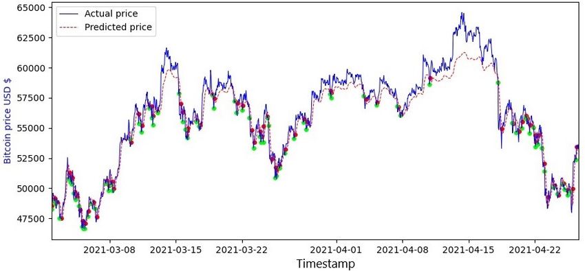
11Figure 4: The real and predicted price from the LSTM model and the best
performing threshold value. Green circle indicates a purchase, and red a sale.
In figure 4 all the trades of the LSTM model using the best threshold
value can be seen. The price of the BTC versus the price of the predicted
price from the LSTM model is also represented in the plot.
4.2 Moving Average
The moving average model ran on the entire data set for all combinations of
hyperparameters presented in the method section. That is, 4 × 3 × 4 = 48
configurations. The most interesting results are presented below. The blue
line in the graphs are the profits over time. The red line is the same for
every run, and represents the BTC price. The titles over the plots show
which hyperparameters that were used. B is ∆, LT is LA and ST is SA.
12(a) (b)
Figure 5: Results for two MA simulations
(a) (b)
Figure 6: Results for two MA simulations
(a) (b)
Figure 7: Results for two MA simulations
134.3 Random Intervals
The random interval bot performed differently every run due to its random
elements. Hence, the profitability varied between the runs. The performances
are presented in histograms, which can be seen below. The yellow dashed
lines are bell curves with the same mean and standard deviations as the
data in the respective histogram. The red lines indicate how the BTC price
changed during the corresponding time period. It shows how much you would
earn or lose by buying a BTC in the beginning of the time period and sell it
at the end of the time period. First, the model ran 1000 times on the entire
data set from 2017. The profitability histogram can be seen in figure 8.
Figure 8: The random interval bot’s profitability for 1 000 runs
The model also ran 5 000 times each on three shorter periods. Histograms
for these months can be seen in figures 9, 10 and 11.
14Figure 9: Profitability histogram for February 2018
Figure 10: Profitability histogram for April 2018
15Figure 11: Profitability histogram for November 2018
The average profitability for every time period as well as the BTC price
change can be seen in table 2
Table 2: Average profitability and BTC price changes
Time Period Average profit [USD] BTC price change [USD]
2017 - 2021 25 915 53 239
February 2018 112 46
April 2018 1 129 2319
November 2018 -1 172 -2 330
5 Discussion
5.1 LSTM
When reviewing the data from the LSTM-model a few conclusions can be
made. At figure 3 the graph shows the profits versus the market performance
for each threshold value. From this graph it appears that when the thresh-
old value is over 0.03 the profits made from the LSTM model are negative,
compared to the market performance. However, when the threshold value
is 0.03 and below, the LSTM model often outperforms the market. Thus
these results seems to imply that when lowering the threshold value, and
16therefore increasing the frequency of the trades, it also increases the chance
of higher profit. As seen in figure 4, the machine learning model predicts the
price relatively well, with a few exceptions, compared to the market. This
indicates that the model predicts the market behaviour relatively well and
has the potential to capitalize on these predictions.
There are a few things that could be tested in order to further improve the
model. One way would be to test using assymetrical values on the thresh-
olds. This would mean that it would require different values for buy and sell
decisions in equation 3. For a more advanced improvement the system could
adapitvely choose a threshold value based on the volatility of the market. For
example, if the market is in a steady state, it would make little sense to trade
in a high frequency. However, if the market is more volatile then it is pre-
sumably advantageous to trade in a higher frequency. Another improvement
would be to include social signals as input in the LSTM model. This could
be done in a number of different ways. One way would be to measure the
search count for different cryptocurrencies, and in that way draw conclusions
on the current popularity of the currency. These signals could offer another
type of data which interprets the market sentiment and could indicate an
upcoming rise or decline.
5.2 Moving average
When reviewing the simulations from the moving average model, a few graphs
were selected to display the key differences. When tweaking the hyperparam-
eters in the model, we see that it is resulting in different outcomes over the
same time period. When using a more narrow bandwidth ∆ the model is
more active, and benefits from the relatively small market fluctuations be-
tween 2018 and the end of 2020. However, this comes with the trade off, larger
market movements are often bypassed - The model sells too early. This can
be seen in figure 5a where the model outperforms the market at first, but
misses out on the large upswing at the end of 2020. At the other end of the
spectrum we have the models that use a broader bandwidth. These models
are unable to operate effectively when the market is more stable, but handle
larger market movements better. This can be seen in figure 7b and 6a. The
model with the most all-round parameters are displayed in figure 7a. This
set of hyperparameters was profitable at the beginning of the data set, but
also manages to hang on when the market rushed upwards in the end of 2020.
17An improvement to the model could be to use an adaptive bandwidth based
on the volatility of the market. This would enable the model to predict both
small and large market movements. This could be done by measuring the
standard deviation in the data, compared to the market volatility. This is a
method commonly used in technical analysis.
5.3 Random intervals
The results from the random interval model seems to imply that it’s most
likely to make a profit even though the the timestamps where to buy and
sell is chosen at random. This is because the overall direction of BTC was
upward between 2017 and 2021. Another observation from figure 8, is that
the market delta was 53239 USD, while the expected value of the wallet delta
was around 22000 USD. This is probably due to that the model was idle for
approximately half of the simulation time and invested for the other half.
Therefore it is most likely that the gain or loss from the model is half of the
market performance.
6 Conclusion
This project has analyzed and investigated the profitability of autonomous
trading in BTC. The conclusion that can be drawn from the various results
is that autonomous trading has potential to be profitable. Though, there
are still difficulties with adapting the models to a real market. Choosing the
appropriate parameters depending on the market behaviour is of the utmost
importance, but remains a challenging task. This task is yet to be fulfilled,
and remains a topic of further research.
18References
[1] James Chen. Amsterdam Stock Exchange (AEX) .AS Definition. 2019.
url: https://www.investopedia.com/terms/a/aex.asp.
[2] Satoshi Nakamoto. Bitcoin: A Peer-to-Peer Electronic Cash System.
2008. url: https://bitcoin.org/bitcoin.pdf.
[3] Ludvig Öberg. Interview with Ludvig Öberg, Co-founder of Safello and
an expert within cryptocurrencies. 2021-04-16.
[4] Christopher Olah. Understanding LSTM Networks. 2015. url: https:
//colah.github.io/posts/2015-08-Understanding-LSTMs.
[5] Jason Brownlee. The 5 Step Life-Cycle for Long Short-Term Memory
Models in Keras. 2017. url: https://machinelearningmastery.com/
5-step-life-cycle-long-short-term-memory-models-keras/.
[6] Binance. Kline/Candlestick Data. url: https : / / binance - docs .
github.io/apidocs/delivery/en/#kline-candlestick-data.
[7] Preprocessing data. url: https : / / scikit - learn . org / stable /
modules/preprocessing.html.
[8] Time series / date functionality. url: https://pandas.pydata.org/
pandas-docs/stable/user_guide/timeseries.html.
[9] Jason Brownlee. Gentle Introduction to the Adam Optimization Algo-
rithm for Deep Learning. 2021. url: https://machinelearningmastery.
com/adam-optimization-algorithm-for-deep-learning/.
[10] Murat Karakaya. LSTM: Understanding the Number of Parameters.
2020. url: https : / / medium . com / deep - learning - with - keras /
lstm-understanding-the-number-of-parameters-c4e087575756.
19You can also read