DYNAMIC PRICING WITH UPDATED DEMAND FOR THE SPORTS AND ENTERTAINMENT TICKET INDUSTRY
←
→
Page content transcription
If your browser does not render page correctly, please read the page content below
Journal of Computer Science 10 (11): 2240-2252, 2014
ISSN: 1549-3636
© 2014 Phumchusri and Swann, This open access article is distributed under a Creative Commons Attribution
(CC-BY) 3.0 license
doi:10.3844/jcssp.2014.2240.2252 Published Online 10 (11) 2014 (http://www.thescipub.com/jcs.toc)

      DYNAMIC PRICING WITH UPDATED DEMAND FOR THE
       SPORTS AND ENTERTAINMENT TICKET INDUSTRY
                                     1
                                         Naragain Phumchusri and 2Julie L. Swann
                                              1
                                              Department of Industrial Engineering,
                              Faculty of Engineering, Chulalongkorn University, Bangkok, Thailand
                                2
                                  H.Milton Stewart School of Industrial and Systems Engineering,
                                     Georgia Institute of Technology, Atlanta, Georgia, USA

     Received 2014-03-06; Revised 2014-03-07; Accepted 2014-11-11
                                                       ABSTRACT
     Revenue Management (RM) helped increase profitability for many travel industries. Selling perishable
     products with a fixed event date, the Sports and Entertainment (S&E) ticket industry can potentially
     benefit from RM ideas but has received less attention in the literature. In this study we develop
     dynamic pricing models for stochastic S&E demand in a discrete finite time setting, where demand
     depends not only on ticket prices but also on remaining times until the show dates. We assume the
     show popularity is uncertain to the seller, but this information can be learned via Bayesian updates as
     early sales are revealed. We present stochastic dynamic programs for Sports and Entertainment tickets
     pricing decisions. We test the models using real data obtained from a major performance venue in the
     U.S. to understand properties of the model solutions and performance under different scenarios. Our
     results show that demand learning is most beneficial when the initial estimates are incorrect. In
     addition, we found it is less necessary for the seller to vary price every period if demand variation is
     low and/or a large amount of demand arrives close to the show dates. Overall, we found that the
     benefits from having flexibility of price changes and demand learning can complement each other to
     achieve as much as 8.15% revenue increase on average, as compared to static pricing.

     Keywords: Dynamic Pricing, Demand Learning, Bayesian Updates, Sports and Entertainment Industry

                      1. INTRODUCTION                                lines (Ladany and Arbel, 1991), passenger railways
                                                                     (Ciancimino et al., 1999) and rental car companies
    Revenue Management (RM) has attracted much                       (Carol and Grimes, 1995; Geraghty and Johnson, 1997).
attention and been proven as one of the most effective               Ultimately, RM is used to support decision making to
practices to increase profitability for many industries.             achieve the goal of selling the right amount of product at
RM first emerged in the airline industry in the context of           the right price to the right customers at the right time
passenger booking problems (Belobaba, 1987;                          (Bitran and Caldentey, 2003).
Littlewood, 1972; Rothstein, 1971). Then, it has played                  Dynamic pricing is an RM tool that is widely used
important roles in improving the performance of many                 to manage and control demand at different points of
industries, selling fixed perishable capacity with high              time. Sellers adjust prices to increase or decrease
set-up costs such as hotels (Bitran and Gilbert, 1996;               demand in the short run so that it can be matched with
Bitran and Mondschein, 1995; Lieberman, 1992), cruise                their available resources. The main objective of
Corresponding Author: Naragain Phumchusri, Department of Industrial Engineering, Faculty of Engineering, Chulalongkorn University,
                      Bangkok, Thailand
    Science Publications
                                                              2240                                                           JCS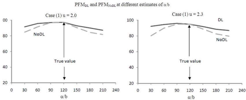
Naragain Phumchusri and Julie L. Swann / Journal of Computer Science 10 (11): 2240-2252, 2014

dynamic pricing is to find an optimal dynamic policy to                     For new products (without past sales information)
balance utilization of the available capacity so that the               and/or products whose demand patterns may deviate
revenue can be maximized over the selling period.                       significantly from past history, demand characterization is
There are extensive papers exploring a variety of                       difficult (Lan et al., 2008). Likewise, the S&E demand can
dynamic pricing topics (Biller et al., 2005; Chan et al.,               be uncertain, especially for a new show or a sports team
2004; Gallego and van Ryzin, 1994; 1997; Kannan and                     with varying performance. So, the seller cannot totally
Kopalle, 2001; Leloup and Deveaux, 2001; Levin et al.,                  rely on past sales history when predicting demand. Early
2009; Maglaras and Meissner, 2006). While dynamic                       sales observations can be useful for demand information
pricing has been intensively studied in the travel                      updates. For example, after the selling time starts, the
industries, the Sport and Entertainment (S&E)                           ticket sellers will have a clearer picture whether the games
industry is another business that has potential to be                   (or shows) are likely to have high or low sales. In this
                                                                        study, we consider stochastic S&E ticket demand and
improved by the idea but still has not received as
                                                                        incorporate demand learning with Bayesian updates. A
much attention (Drake et al., 2008).
                                                                        stochastic setting is appropriate to capture real-life
    There are approximately 1,953 sport stadiums and
                                                                        situations when the paths of demand over time is difficult
236 performance venues in the United States, with the
total revenue of 44.2 billion reported in 2009                          to be accurately predicted (Bitran and Caldentey, 2003);
(PricewaterhouseCoopers, 2010). Similar to the airline                  while demand learning allows the seller to update his
business, the number of the S&E tickets is fixed and they               beliefs as uncertainty reveals itself.
are “perishable” since they have no value after the event                   In this study, we assume ticket demand in each
date. However, the S&E industry’s characteristics differ                period follows a Poisson distribution, where its rate is
from airlines or hotels in many ways. First, a much                     affected by three components; (1) the artists/sport
higher percentage of entertainment tickets are purchased                teams’ popularity, (2) the ticket price and (3) the
on the day of the show than on the day of a flight or on                remaining time until the show date. Including timing
the day of a hotel stay (Drake et al., 2008). Secondly,                 effects for the S&E ticket demand is motivated by the
while important factors of demand are date/time of a                    actual data. Figure 1 depicts the average number of
flight for airlines and day/month of a stay for hotels, the             tickets sold for 108 shows performed in a major
S&E ticket demand is also very related to the sport teams               performance venue in the U.S. during the 2007-2008
or performance artists’ popularity. Moreover, consumer                  season, where the horizontal axis represents the number
tastes and economic conditions change over time and                     of months prior to the show dates. The upper and lower
events vary from one year to another, so it is difficult to             lines represent the average plus and minus one standard
incorporate all uncertainties to precisely predict S&E                  deviation, respectively. We can see in Fig. 1 that the
ticket sales. For these reasons, a different pricing model              average number of seats sold each month is dependent
is necessary for the S&E industry.                                      on time prior to the show and it generally increases
    Although there are a number of studies that are related             when the time is closer to the event date.
to ticket pricing (Courty, 2003; Deserpa, 1994; Rosen and                   In our demand model, the seller can characterize
Rosenfield, 1997) and the topic of price variation in the               price effects and timing effects on demand, but he has
S&E business (Leslie, 2004; Rascher, 1999), the previous                incomplete information about the event popularity (i.e.,
research considered static pricing decisions where ticket               the base demand rate). The seller forecasts the base
prices remain constant for the entire selling horizon. It is            demand rate’s initial estimation and then uses the
generally because in the past, most event tickets were sold             observed sales to update his belief about the upcoming
with a fixed price (independent of when the tickets were                period’s demand. We develop dynamic pricing models in
sold) due to the limited inventory tracking devices or                  a discrete-finite-time selling horizon. In the first period,
ticket changes were done on an ad-hoc basis. However, in                the seller determines the optimal base ticket price. In the
recent years, tools such as internet based selling systems              following periods, the seller can offer discounts
have become widely available, providing information for                 (decrease price) or charge premiums (increase price),
real-time demand observations. From our discussions with                with respect to the decided base price. We develop a
a performing arts consulting firm, there has been a                     dynamic pricing model in a discrete-finite-time selling
significant interest from a number of performance arts                  horizon. In the first period, the seller determines the
organizations for methods to apply dynamic                              optimal base price. In the following periods, the seller can
discounts/premiums pricing to more effectively manage                   offer discounts (decrease price) or charge premiums
demand and increase revenue.                                            (increase price), with respect to the decided base price.

    Science Publications                                         2241                                                          JCS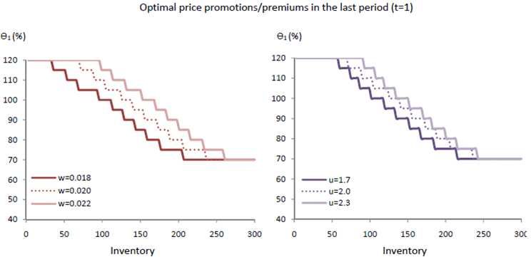
Naragain Phumchusri and Julie L. Swann / Journal of Computer Science 10 (11): 2240-2252, 2014

We develop a method for pricing and learning that allows                                         Θt ( pt ,Γt ) = φ ( pt ) g (t ) Γt
us to address the following research questions:
                                                                        where, φ (pt) represents price effects (i.e., the probability
•   How can the observed sales be used in the demand                    of each arrival purchasing a ticket) and it is decreasing
    learning process to improve the forecast and when is                with price pt. The demand timing effect, g(t), is a
    demand learning most beneficial?                                    decreasing function of t (where t = n at beginning of the
•   How are the optimal price changes related to model                  selling time and t = 0 at the show/event time). This
    parameters such as price sensitivity and remaining                  assumption is underlined from the data we observed
    inventory of unsold tickets?                                        (Fig. 1) that ticket demand tends to increase closer to the
                                                                        show date. Also, ticket demand is sensitive to price,
    This study is organized as follows. We begin by we                  which is intuitive.
discussing demand assumptions and describe how the                          From our discussions with the performing arts
observed sales are used to update the belief about the                  consulting firm, the show’s popularity in customers’
upcoming period’s demand in the learning process.                       perspective is usually uncertain to the seller. It is usually
Section 3, we present the dynamic discounts/premiums                    difficult to correctly forecast demand. Therefore, in our
pricing model, where the price discounts/premiums                       model we assume there is incomplete information on the
adjustment is allowed in every period and discuss the                   exact value of the base demand rate, Γt. At the beginning
value of applying demand learning to the pricing model                  of the selling time (t = n), we assume Γn follows a
via the computational study. Finally, Section 4 concludes               Gamma distribution with a scale parameter of a and a
with a summary of insights from the results this study
                                                                        shape parameter of b. In addition to the show’s
and discusses interesting future research ideas that this
study could be extended further.                                        popularity, a and b may depend on the city in which the
                                                                        show is performed, since we may expect a higher base
       2. DEMAND LEARNING MODEL                                         demand rate for the show taking place in a bigger city. A
                                                                        Gamma distribution allows the flexibility of the shape
    In this section, we describe our demand model and                   and position to be changed extensively via parameters a
show how the observed sales are used to update beliefs                  and b, where empirically we found it a good match to
about demand in the upcoming periods.                                   past data. Let Mn be the random demand in period t = n.
    In this model, the ticket demand in each period t is                The distribution of Mn, conditional on the base demand
assumed to follow a Poisson process with rate Θt(pt, Γt),               rate (Γn = γ) and ticket price (pn), follows a Poisson
which is affected by three components: (1) the ticket                   distribution with rate φ (pn)g(n)γ. Thus, for demand in
price, (2) the artists/sport teams’ popularity and (3) the              the first period, we have Equation 1:
remaining time until the show date. Note that pt denotes
the ticket price in period t and Γt denotes the base                    f ( M n = m | Γ n = γ , pn )
demand rate, which represents the expected popularity of                    [φ ( pn ) g (n)γ ]m e −φ ( pn ) g ( n )γ                       (1)
                                                                        =                                            , ∀m ∈ {0,1, 2,...}
the show. The overall demand rate is defined as follows:                                   m!

Fig. 1. The average ticket sales of 108 shows performed in a major performance venue in the U.S. during the 2007-2008 season, at
        different times prior to the show

    Science Publications                                         2242                                                                      JCS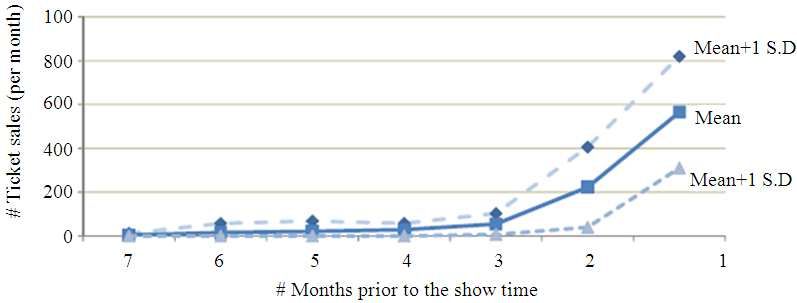
Naragain Phumchusri and Julie L. Swann / Journal of Computer Science 10 (11): 2240-2252, 2014
Similarly, the distribution of demand in period t f (M n -1 = m | pn -1 , pn , mn )
(denoted by), conditional on the base demand rate ∞
= ∫ f ( M n -1 = m | Γ n -1 = γ, pn -1 ) f (γ | pn , mn ) dγ
and ticket price, follows a Poisson distribution 0
m -φ ( pn-1 )g( n -1)γ
with rate, i.e., Equation 2: ∞ [φ ( pn -1 )g( n - 1)γ] e
= ∫ 0
(
m!
)
[φ ( pt ) g (t )γ]m e-φ ( pt ) g (t )γ e-γ[b+φ ( pn )g(n)]γ a + mn -1[b + φ ( pn )g(n)]a + mn
f ( M t = m | Γt = γ, pt ) = , ×( )dγ
m! (2) (a + mn -1)!
∀m ∈ {0,1, 2,...}, ∀t ∈ {n -1,...,1} m + a + mn - 1 φ ( pn -1 ) g (n - 1)
m
=
m b + φ ( p n ) g ( n ) + φ ( p n -1 ) g ( n - 1)
Next, we identify the prior distribution of the demand in α +m n
b + φ ( pn )g( n)
the first selling period (t = n). From Bayes’ rule, we have × , ∀m ∈ {0,1, 2,...},
b + φ ( p ) g ( n ) + φ ( p ) g ( n - 1)
that the distribution of demand (when the price is pn), n n -1
unconditional on τn, is given by Equation 3:
where, f(Mn-1= mΓn-1=γ,pn-1) is given by (2) for tn-1 and
f(γmn, pn) is the distribution function of Γn-1, given by
f ( M n = m | pn )
∞
(4). We can see that Mn-1 follows a Negative Binomial
= ∫ f ( M n = m | Γ n = γ, pn ) f (γ)dγ
0
distribution with parameters α+mn and
-φ ( pn ) g ( n )γ α -1 α b + φ ( pn ) g ( n )
[φ ( pn ) g (n)γ] e
m -bγ
∞ e γ b . From the demand functions
= ∫
0
(
m!
)(
(α - 1)!
) dγ (3) b + φ ( pn ) g ( n) + φ ( pn -1 ) g ( n - 1)
m α described above, we find that the base demand rate and the
m + a - 1 φ ( pn ) g ( n ) b unconditional ticket demand distributions in any period t
=
m b + φ ( p n
) g ( n ) b + φ ( p n
) g ( n ) can be summarized in the following Theorem.
∀m ∈ {0,1,2,...}
Theorem 1
In period t, where n 0
(a + mn -1)!
f ( M t = m | pt , pt +1 ,..., pn , mt +1 ,..., mn )
n
m + a + ∑ mk - 1 φ ( pt ) g (t )
m
Thus, the posterior distribution of Γn-1 at the
=
k = t +1
A(t )
beginning of the next period (t = n-1) follows a Gamma
m
distribution with a scale parameter of a +mn and a shape n
parameter of b + φ (pn)g(n). b + ∑ n φ ( pk ) g ( k )
a+ ∑
k =t +1
nk
From Bayes’ rule, the distribution of demand in × k = t +1
, ∀m ∈ {0,1, 2,...}
A(t )
period t = n-1 is given by:
Science Publications 2243 JCS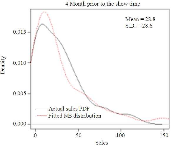
Naragain Phumchusri and Julie L. Swann / Journal of Computer Science 10 (11): 2240-2252, 2014

where, A(t ) = b + ∑ k = t +1φ ( pk ) g (k ) + φ ( pt ) g (t ) . Note that          price discounts/premiums adjustments are allowed in
                            n

                                                                                    every period, in the context of a stochastic dynamic
ticket demand takes non-negative integer values. The                                program in section 3.1. Computational analysis is then
posterior Negative Binomial distribution of demand is                               presented in section 3.2 to provide insights on the
advantageous since it provides the probability mass function                        optimal pricing structures and the benefit of demand
for non-negative integers. Moreover, the shape and position                         learning for the described pricing model.
can be changed extensively via its two parameters
(Subrahmanyan and Shoemaker, 1996). From ticket sales                               3.1. Model
data of the 2007-2008 season obtained from a performance                                We consider a discrete finite time setting, where there
venue in the U.S. (108 shows), Fig. 2 depicts the probability                       are n sub-periods from the beginning of the selling horizon
density plots of sales occurred at different times in the                           to the event/show time. The time periods are numbered in
selling horizon; i.e., one, two, three and four months prior to                     reverse chronological order so that the beginning of the
the show time, respectively. Using the Maximum-                                     selling horizon is time t = n and the show takes place at
Likelihood method, the actual data was fitted to the                                time t = 0. At the beginning of the selling horizon (t = n),
Negative Binomial distribution, where the fitted values of                          there are In number of tickets for sale. The number of
mean and standard deviation were shown. From the                                    tickets demanded and the actual sales in period t are
Pearsons Chi-Square test (Plackett, 1983), we found that                            denoted by dt and mt, respectively. If demand is less than
with a significant level of 5%, the hypothesis that demand                          inventory at the beginning of period, It, the ticket sales in
(from the venue’s data) follows a Negative Binomial                                 period t(mt) are equal to dt. However, if demand exceeds
distribution was accepted for all graphs shown in Fig. 2.                           inventory (dt>It), the ticket sales mt will equal It.
     Given the observed sales data, the seller updates his                              In the first period of the selling horizon (t = n), the
belief about demand in the next period. The following                               seller determines the base price, pn. Then, at time t = n-
Proposition presents the relationships between the                                  1,…,1, the seller observes past sales and decides whether
expected demand and key relevant factors.                                           to offer any discounts (reduce price) or charge premiums
                                                                                    (increase price) and how much. Denote θt as the discount
Theorem 2                                                                           or premium for period t and we assume it is based on pn,
    The expected demand in period t is:                                             (i.e., customers pay θtpn for each ticket in period t). If
                                                                                    θt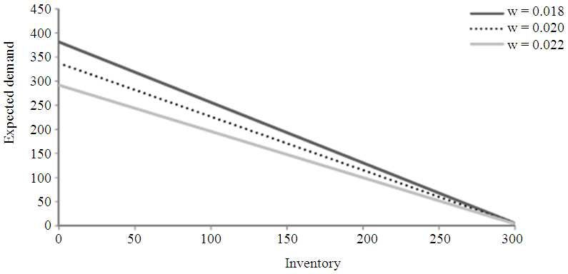
Naragain Phumchusri and Julie L. Swann / Journal of Computer Science 10 (11): 2240-2252, 2014
α n min{I n , d n (α n )} = pn min{I n , d n ( pn )} Let the timing effect be g(2) = 1 and g(1) = u, (where
if t = n; u>1 since we assume higher demand in the period closer
Rt (α t ) =
α t pn min{I t , dt (α t )} = θt pn min{I t , dt (θt pn )} to the show date). At the beginning of the selling horizon
if t = n -1,...,1, (t = 2), the seller believes that ticket demand is Poisson,
with the base rate (Γ2) following a Gamma distribution
where, it = max{0, lt+1-dt+1(αt+1)} The boundary with parameters a = 4 and b = 0.04 (This choice of a and b
conditions are as follow Equation 6 and 7: follows from an example of actual ticket demand data we
observed). In this period (t = 2), the seller determines the
V0 (h0 ) = 0, ∀h0 (6)
optimal base ticket price, p*2 , from a discrete set P2={30,
Vt (ht = (ht +1, at +1, mt +1,0)) = 0,"t
(7) 35, . . . , 75, 80}. After he observes how many tickets have
been sold, the seller updates his belief with demand learning
Condition (6) means there is zero salvage value of any techniques presented in section 3 and determines the
unsold tickets at the event time (t = 0 ). Condition (7) states optimal price discount/premium, θ1* , to charge in period t =
that when all tickets have already been sold, the revenue
1 from a discrete set θ1={70%, 75%, . . . , 115%, 120%}.
from any period t on is zero since there are no tickets left for
Figure 3 presents the updated mean demand for
sale. The stochastic dynamic program can be solved by
period t = 1 at different values of remaining inventory
backwards induction starting at the final period, t = 1, to
from the past period (where the price sensitivity
period t = n. The following example is a special case where
parameters (w) equal 0.018, 0.020 and 0.022,
the selling time is divided into two periods, n = 2.
respectively (Parameter values for the price sensitivity
3.2. Computational Experiments parameters (w) in this experiment result in shifts of
0.9%-1.1% (at p1 = 50) which is consistent with data we
In this section, we perform computational experiments
have seen). As expected, at the same values of remaining
for the dynamic discounts/premiums pricing model, with
inventory, the graph for w = 0.018 is the highest and the
the goal of understanding the properties of the optimal
graph for w = 0.022 is the lowest in Fig. 3, since a higher
solutions and the model performance under different
price sensitivity leads to lower expected demand.
situations. Specifically, we consider: (1) How the
Moreover, considering the trends, we can see that the
remaining inventory affects the expected base demand
higher number of tickets left in inventory (i.e., the lower
rate and the optimal discounts/premiums pricing policy
number of tickets already sold), the lower mean demand
and (2) how the performance of the dynamic
the seller expects for the next period. This is consistent
discounts/premiums pricing model with demand learning
with analytical results in Theorem 2 (iii) in Section 3 that
is compared to the model without demand learning and
the expected mean demand is increasing with observed
when demand learning is most beneficial.
sales in the past periods (so it is decreasing with the
3.3. Effects of the Remaining Inventory of leftover inventory). The finding is rational because
Unsold Tickets having a large number of tickets sold in the past periods
(or a few number of tickets left in the inventory) can be
In each period, the seller can observe how many an indicator of show popularity and it is likely that high
unsold tickets remained in inventory. This section demand will occur in the next period as well.
explores how the seller’s expectation and optimal We solve the described problem by the stochastic
decisions are affected by the inventory information. Let dynamic program described in section 4.1. The optimal
us consider the following example. A ticket seller has base price at the beginning of the selling horizon (t = 2)
300 tickets for sale in a selling season with n = 2. Let the is 95. After sales are realized, the seller’s optimal
probability of each arrival purchasing a ticket (the price discount/premium pricing for period t = 1 is shown in
effect function) be φ (pt) = e-wpt, where w is a known non- Fig. 4, where the horizontal axis represents different
negative scalar. Note that with this form of price effect, values of leftover inventory, I1. Note that different lines
the demand rate equals g(t)Γt when pt equals 0 and the rate in Fig. 4a represent different price sensitivity
approaches 0 as pt is very large. This form of exponential parameters, i.e., w equals 0.018, 0.020 and 0.022,
price effect function has been generally used in the respectively; while different lines in Fig. 4b represent
marketing literature since it was found to very well fit with different timing effect parameters, i.e., u equals 1.7,
the empirical data (Aviv and Pazgal, 2002). 2.0, 2.3, respectively.
Science Publications 2245 JCS
Naragain Phumchusri and Julie L. Swann / Journal of Computer Science 10 (11): 2240-2252, 2014

Fig. 2. The probability density plots of ticket sales from a major performance venue in the U.S. (during the 2007-2008 season)

                  Fig. 3. The expected demand for the last period (t = 1) at different values of remaining inventory

Science Publications                                            2246                                                        JCS
Naragain Phumchusri and Julie L. Swann / Journal of Computer Science 10 (11): 2240-2252, 2014

                                       (a)                                                        (b)

Fig. 4. The optimal discounts/premiums pricing for the last period (t = 1) at different values of leftover inventory, where (a) w =
        0.018, 0.020, 0.022 (b) u = 1.7, 2.0 and 2.3, (a) at different price sensitivities (where u = 2) (b) at different timing effects
        (where w = 0.020)

Observation 1                                                           learning. The insights will allow us to identify which
                                                                        situations are most worthwhile to apply the learning
    The optimal ticket price discount/ premium,θt, is                   process. The Demand Learning (DL) model incorporates
nonincreasing with the amount of leftover inventory                     observed sales in updating the belief of the next period’s
observed at the beginning of the period.                                demand, while the No Demand Learning (NoDL) model
    Similar to other sets of experiment results we have                 does not. Thus, when the seller applies the NoDL model,
explored, Observation 1 states that the higher the                      in every period he uses the same estimated base demand
inventory, the lower the percentage of the base price that              rate as in the first period. We capture the DL and the
should be charged in the last period (t = 1). This result is            NoDL model performances by comparing revenues
consistent with other studies of dynamic pricing with no                obtained from each model to the revenue under perfect
demand learning where the optimal price is found to be                  information. Note that under perfect information, the
non-increasing with the remaining inventory (Chatwin,                   seller knows the true base demand without uncertainty
2000; Feng and Xiao, 1999; Zhao and Zheng, 2000). In                    and he optimizes his prices based on the true value.
addition, we can see in Fig. 4a that at the same level of               Define PFMDL as the performance of demand learning,
inventory, the higher the price sensitivity, the lower the                                   Re venue of demand learning mod el
optimal θ1. The timing effect parameter (u) also impacts                i.e.,     PFM DL =                                         × 100
                                                                                             Re venue of perfect inf ormation case
the optimal θ1. From Fig. 4b, at the same inventory level,
the line with u = 2.3 is the highest and the line with u =              and PFMNoDL as the performance of the no demand
1.7 is the lowest It implies when high demand is                        learning               model,               i.e.,
expected in the last period, it is less necessary for the                            Re venue of demand learning mod el
                                                                        PFM NoDL =                                         × 100
seller to offer a deep discount (since there is a lower risk                         Re venue of perfect inf ormation case
of having empty seats).                                                     The closer PFMDL and PFMNoDL are to 100, the better
    Next, we examine benefits of demand learning and                    their performances are as compared to the perfect
identify which situations are most worthwhile for
                                                                        information case, although the latter may not be achievable.
applying the learning process.
                                                                            Consider a ticket seller having 100 tickets for sale in
3.4. Benefits of Demand Learning Process                                a two-period selling horizon, where the timing effects are
                                                                        g(2) = 1 and g(1) = u, u>1. The price effect function is
    In this section, we study how the performance of the                φ (pt) = e-0.02pt. At the beginning of the selling time (t =
dynamic discount/premium pricing model with demand
learning compares to the model without demand                           2), the seller determines the optimal base ticket price, p*2 ,

    Science Publications                                         2247                                                              JCS
Naragain Phumchusri and Julie L. Swann / Journal of Computer Science 10 (11): 2240-2252, 2014
from a discrete set P2 = {50, 55, . . . , 95, 100}. Then in Observation 2
the next period (t = 1), he determines the optimal price
We found that:
discount/premium ( θ1* ) from a discrete set Θ1 = {70%,
75, . . . , 115, 120%}. • Demand Learning (DL) is most beneficial, as
Let us consider what happens if the ticket seller compared to No Demand Learning (NoDL) when
misestimates demand. For instance, suppose the true the initial estimation is inaccurate (with up to 8-
base demand rate in the first period (t = 2) is γ, while the 11% improvement in revenue when the
seller believes the base demand rate follows Gamma misestimates are high)
distribution with parameters a and b, respectively. Note • The marginal benefit of the DL model over the
that the expected value of the base demand rate in this NoDL model is higher when a greater amount of
α α demand arrives in the last period (approximately
case equals and the variance equals (for Gamma
b b2 5.4% improvement in revenue on average for case 2,
distribution). Thus, the demand is overestimated if the as compare to 3.9% for case 1)
α • The underestimation of the base demand rate when
seller believes that is greater than the true base demand using the DL model causes fewer revenue loss as
b
rate, γ and the demand is underestimated otherwise. compared to overestimation
In the following example, let the true base demand
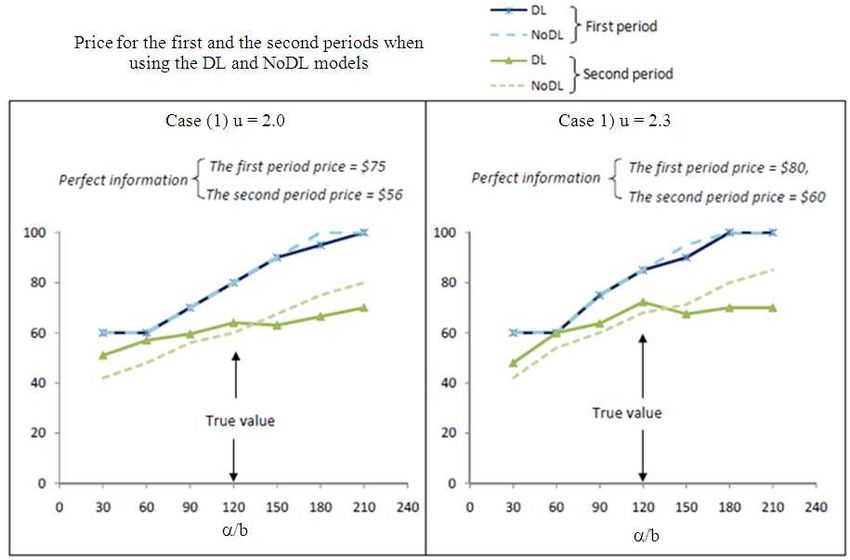
rate, γ, be 120. Fig. 5 shows the chosen prices for the As we can see in Fig. 6, when the misestimates of the
first and the second periods when the seller’s estimates base demand rate are fairly large, PFMDL is greater than
α PFMNoDL for both graphs. It implies demand learning can
of the mean base demand rate ( ) are 30, 60, . . . , 210, help increase revenue, compared to no learning. The
b
240, respectively. The second period (t = 1) price equals intuition is that when there are estimation errors,
the first period (t = 2) price times the discount/premium observed sales are effectively used since the inaccurate
estimation can be corrected for an updated belief of
of the second period (p1 = p2 × θ1). In case 1, u = 2.0 and
demand in the next period. For example, if there is high
the optimal prices under perfect information are 75 and
uncertainty about the show’s popularity (e.g., a new
56 for the first and the second period (in case 2 with u =
show with no records of past sales), it can be difficult for
2.3, they are 80 and 60, respectively). We can see from
the ticket seller to identify a correct value of the show’s
Fig. 6 that in the first period, both DL and NoDL models
base demand rate. The seller can start with a rough
α
choose similar prices for almost all values of . estimate of the base demand rate and then use the
b
observed sales to update his belief.
However, when the base demand rate is underestimated, In addition to the demand pace, we observe that
α
i.e., < 120 , the DL model’s prices for the second demand learning affects the performance difference
b between the two models. Specifically, the dynamic
period are higher than the NoDL model’s. Due to the timing model’s performance is closer to the dynamic
ability of updating demand, the DL model uses the discounts/premiums pricing model’s when demand
observed sales to adjust the true base demand rate’s learning is not allowed (as PFMDT is closer to 100 in this
distribution for the next period. With the DL model, case). It indicates limiting the frequency of price changes
the seller realizes in the second period that he has is less disadvantageous, compared to allowing price
underestimated the rate and then decides to charge changes every period, when the seller does not use
higher prices than he would have done without observed sales to update his belief of demand. An
Demand Learning (NoDL). Similar reason applies explanation is when the seller allows demand learning,
when the base demand rate is overestimated, where new information is received every period. So, it can be
the second period’s prices chosen by the DL model more beneficial to change price often, according to the
are lower than the NoDL model. updated demand. Adjusting price regularly as in the
Considering the performance of each model, Fig. dynamic discounts/premiums pricing model can lead to
6. shows PFMDL and PFMNoDL, where the horizontal higher revenue, especially with an integration of demand
α learning implementation. This observation is consistent
axis represents different estimates of and the true
b with results across the set of computational experiments
value is indicated. we performed, using different demand parameters.
Science Publications 2248 JCSNaragain Phumchusri and Julie L. Swann / Journal of Computer Science 10 (11): 2240-2252, 2014
Fig. 5. The optimal prices for the first and the second periods when using the DL and the NoDL models
α
Fig. 6. Performances of the DL and the NoDL models at different estimates of , when the timing effects, u, are 2.0 (the left
b
diagram) or 2.3 (the right diagram)
Science Publications 2249 JCSNaragain Phumchusri and Julie L. Swann / Journal of Computer Science 10 (11): 2240-2252, 2014
Fig. 7. The average percentage revenue increase(from static pricing policy) under different scenarios
We conclude this section by exploring the benefit We found that the optimal price discount/premium for
gained from dynamic pricing as compared to static the upcoming period is non-increasing with the amount of
pricing. Figure 7 shows the average percentage revenue remaining inventory observed at the beginning of the
increase from implementing the dynamic discounts/ period. To identify the benefit of demand learning, we
premiums pricing model and the dynamic timing model, compared the described model to a similar model without
with demand leaning and without demand learning, learning. We observed that demand learning is most
respectively. We observe that dynamic pricing (without beneficial when the initial demand estimation is
demand learning) can help increase revenue by inaccurate since the seller can correct his belief after
approximately 3.26-4.33%, compared to static pricing. observing the actual sales (with up to 8-11%
When demand learning is incorporated with one price improvement in revenue when the misestimation is high).
change (dynamic timing model), the average revenue In addition, our results showed: When incorporating
increase is approximately 5.19%. Moreover, we found demand learning, the underestimation of the base demand
that the benefits from having flexibility of price changes rate causes less revenue loss as compared to
(dynamic discounts/premiums pricing model) and overestimation. This implies a risk-averse seller who
demand learning can complement each other to achieve tends to underestimate the demand rate may obtain higher
as much as 8.15% revenue increase. revenue than a risk-taker seller who overestimates it.
It is worthwhile to note that our model is suitable for
4. CONCLUSION situations when ticket demand is sensitive to both price
and time of the selling season, according to our demand
While Revenue Management (RM) has been learning model assumption. A challenging task is to
intensively studied in the travel industries, Sport and identify this function correctly to help this model
Entertainment (S&E) also has a great potential to be compute the suitable ticket price for each selling period.
improved by this idea but still has not obtained much There are several possible extensions of this study. First,
attention in the literature. In addition, there may be our model assumes demand uncertainty comes from the
models or insights from the S&E industry that may base demand rate, while the price and the timing effects
apply to other RM contexts. In this study, we developed are unchanging. One could extend the model to allow
pricing and timing models for stochastic S&E ticket imperfect information on price and/or timing sensitivities
demand in the existence of demand learning with to explore the form of the resulting posterior distribution.
Bayesian updates to reduce uncertainty and improve We expect the distribution will be more complex in those
forecast. We also allow flexibility of demand being cases, but it could be interesting to examine if the benefit
affected by time since in the S&E industry, we can offset the higher complexity. A second promising
observed significantly higher sales when it is closer to extension is a pricing model with demand learning for
the end of the selling horizon. substitutable products, e.g., substitutable seating sections
Science Publications 2250 JCSNaragain Phumchusri and Julie L. Swann / Journal of Computer Science 10 (11): 2240-2252, 2014
or shows. If the ticket seller would like to allow different Chatwin, R., 2000. Optimal dynamic pricing of
discounts/premiums for different types of seats or perishable products with stochastic demand and a
different days of the same performance, it can be useful finite set of prices. Eur. J. Operat. Res., 125: 149-
to study how he can employ the observed sales to predict 174. DOI: 10.1016/S0377-2217(99)00211-8
future demand for a variety of substitutable products Ciancimino, A., G. Inzerillo, S. Lucidi and L. Palagi,
(although there may not exist a closed form posterior 1999. A mathematical programming approach for
distribution for each of them). Another possible the solution of the railway yield management
extension is a dynamic pricing model that allows price problem. Trans. Sci., 33: 168-181. DOI:
adjustment only once. Each period, the seller needs to 10.1287/trsc.33.2.168
decide whether or not he should reduce or increase price Courty, P., 2003. Ticket pricing under demand
and he has only one chance to do so. This model can be uncertainty. J. Law Econ., 46: 627-652. DOI:
applied to situations when adjusting price frequently is 10.1086/377117
costly or not preferable. Deserpa, A., 1994. To err is rational: A theory of excess
Since dynamic pricing is fairly new for the S&E demand for tickets. Managerial Decis. Econ., 15:
business, an empirical work exploring the short-term and 511-518. DOI: 10.1002/mde.4090150513
long-term effects of this revenue management idea could Drake, M.J., S. Duran, P. Griffin and J. Swann, 2008.
be useful. Obviously, there is still room for revenue
Optimal timing of switches between product sales
management improvement for the Sports and
for sports and entertainment tickets. Naval Res.
Entertainment ticket industry and we hope our study will
Logist., 55: 59-75. DOI: 10.1002/nav.20266
encourage future research in this area.
Feng, Y. and B. Xiao, 1999. Maximizing revenues of
5. REFERENCES perishable assets with a risk factor. Operat. Res., 47:
337-341. DOI: 10.1287/opre.47.2.337
Aviv, Y. and A. Pazgal, 2002. Pricing of short life-cycle Gallego, G. and G. van Ryzin, 1994. Optimal dynamic
products through active learning. Working paper. pricing of inventories with stochastic demand over
Washington University in St. Louis. finite horizons. Manage. Sci., 40: 999-1020. DOI:
Belobaba, P., 1987. Airline yield management: An 10.1287/mnsc.40.8.999
overview of seat inventory control. Trans. Sci., 21: Gallego, G. and G. van Ryzin, 1997. A multiproduct
63-73. dynamic pricing problem and its applications to
Biller, S., L. Chan, D. Simchi-Levi and J. Swann, 2005. network yield management. Operat. Res., 45: 24-
Dynamic pricing and the directto-customer model in 41. DOI: 10.1287/opre.45.1.24
the automotive industry. Elec. Commerce Res., 5: Geraghty, M.K. and E. Johnson, 1997. Revenue
309-334. DOI: 10.1007/s10660-005-6161-4 management saves national car rental. Interfaces,
Bitran, G. and S. Gilbert, 1996. Managing hotel reservations 27: 107-127.
with uncertain arrivals. Operat. Res., 44: 15-49. Kannan, P. and P. Kopalle, 2001. Dynamic pricing on the
Bitran, G. and S. Mondschein, 1995. An application of internet: Importance and implications for consumer
yield management to the hotel industry considering behavior. Int. J. Elec. Commerce, 5: 63-83.
multiple stays. Operat. Res., 43: 427-443. Ladany, S. and A. Arbel, 1991. Optimal cruise-liner
Bitran, R. and R. Caldentey, 2003. Pricing models for passenger cabin pricing policy. Eur. J. Operat. Res.,
revenue management. Manufactur. Service Operat. 55: 136-147. DOI: 10.1016/0377-2217(91)90219-L
Manage., 5: 203-229. Lan, Y., H. Gao, M. Ball and I. Karaesmen, 2008.
Carol, W. and R. Grimes, 1995. Evolutionary change in Revenue management with limited demand
product management: Experiences in the car rental information. Manage. Sci., 54: 1594-1609. DOI:
industry. Interfaces, 25: 84-104. 10.1287/mnsc.1080.0859
Chan, L., Z. Shen, D. Simchi-Levi and J. Swann, 2004. Leloup, B. and L. Deveaux, 2001. Dynamic pricing on
Coordination of Pricing and Inventory Decisions: A the internet: Theory and simulations. J. Elec.
Survey and Classification. In: Handbook of Commerce Res., 1: 265-276. DOI:
Quantitative Supply Chain Analysis: Modeling in 10.1023/A:1011546021787
the E-Business Era, Simchi-Levi, D. (Ed.), Kluwer Leslie, P., 2004. Price discrimination in broadway
Academic, ISBN-10: 1402079524, pp: 335-392. theater. RAND J. Econ., 35: 520-541.
Science Publications 2251 JCSNaragain Phumchusri and Julie L. Swann / Journal of Computer Science 10 (11): 2240-2252, 2014
Levin, Y., J. McGill and M. Nediak, 2009. Dynamic Rascher, D., 1999. A Test of the Optimal Positive
pricing in the presence of strategic consumers and Production Network Externality in Major League
oligopolistic competition. Manage. Sci., 55: 32-46. Baseball. In: Sports Economics: Current Research,
DOI: 10.1287/mnsc.1080.0936 Fizel, J., E. Gustafson and L. Hadley (Eds.),
Lieberman, W., 1992. Implementing yield management. Westport, CT: Greenwood, ISBN-10: 0275963306,
ORSA/TIMS National Meeting, (San Francisco, pp: 27-45.
California). Rosen, S. and A. Rosenfield, 1997. Ticket pricing. J.
Littlewood, K., 1972. Forecasting and control of Law Econ., 40: 351-376.
passenger bookings. Proceedings of the AGIFORS Rothstein, M., 1971. An airline overbooking model.
Symposium, (AGIFORS’ 72), pp: 95-117. Trans. Sci., 5: 180-192.
Maglaras, C. and J. Meissner, 2006. Dynamic pricing Subrahmanyan, S. and R. Shoemaker. 1996. Developing
strategies for multiproduct revenue management optimal pricing and inventory policies for retailers
problems. Manufactur. Service Operat. Manage., 8: who face uncertain demand. J. Retail., 72: 7–30.
136-148. DOI: 10.1287/msom.1060.0105 DOI: 10.1016/S0022-4359(96)90003-2
Plackett, R., 1983. Karl pearson and the chi-squared test. Zhao, W. and Y.S. Zheng, 2000. Optimal dynamic
Int. Stat. Rev., 51: 59-72. DOI: 10.1007/978-1- pricing for perishable assets with nonhomogeneous
4612-0103-8_1 demand. Manage. Sci., 46: 375-388. DOI:
PricewaterhouseCoopers, 2010. Official website of 10.1287/mnsc.46.3.375.12063
PricewaterhouseCoopers.
Science Publications 2252 JCSYou can also read