Are LEDs the Next CFL: A Diffusion of Innovation Analysis
←
→
Page content transcription
If your browser does not render page correctly, please read the page content below
Are LEDs the Next CFL:
                                  A Diffusion of Innovation Analysis

                      Christine Holland, Northwest Energy Efficiency Alliance

   ABSTRACT

           This paper examines properties of compact fluorescent lamp (CFL) adoption in the
   Pacific Northwest and early adoption characteristics of light emitting diode lamps (LED) to
   glean similarities and differences. CFLs were the emerging technology in the 90’s competing
   against the dominant incandescent bulb. With the phase-out of incandescent bulbs due to
   Federal legislation (see EISA 2007), within the next few years, CFLs will initially be the
   dominant bulb and LEDs will be the emerging technology. There is much discussion as to
   whether LEDs can reach a price point that will make them cost-effective enough to displace the
   competition. Although there is limited LED data due to its infancy in the market, information
   may be inferred from the more mature CFL market. With 17 years of CFL data, diffusion of
   innovation parameters via Bass model estimation are calculated. Additionally, own-price and
   income elasticities are calculated with more simple logarithmic functions.
           We find that CFLs are highly income elastic with a range of 6.10 to 7.80, implying that
   CFLs are a luxury good. Own-price elasticity ranges from -0.94 to -2.99 supports strong price
   sensitivity. Further, after 17 years, households in the Pacific Northwest have a CFL socket
   saturation of 24% while obtaining a peak market share of approximately 33% of all medium
   screw-based bulbs in 2008, suggesting that many consumers were never reached in this market.
   First cost and quality of CFLs were barriers that were never fully removed to attract these latter
   consumer groups, resulting in lost energy savings potential. LEDs provide the most energy
   saving in the residential lighting market, so from a conservation perspective are highly desirable.
   LEDs are on the right track as their price forecasts show precipitous declines, but may remain 2
   to 3 times higher than CFLs. Therefore, given the evidence of strong consumer sensitivity to
   CFL price, LEDs may not reach their highest possible saturation rate unless prices can drop more
   than expected or non-financial benefits outweigh consumer cost concerns.

   Introduction
           The Energy Independence and Security Act (EISA 2007), phasing out most traditional
   medium screw-based incandescent bulbs over the next two years, has created a new playing field
   for LEDs, CFLs, and Halogen bulbs. LEDs and CFLs will get an additional market boost by a
   ‘second’ phase of EISA which will prohibit the manufacture of general service lamps unable to
   meet an efficacy standard of 45 lumens per watt by year 2020 thus eliminating most Halogens
   from the market (LightBulbChoice.com 2014). Navigant Consulting, Inc. and SAIC (2012)
   imply that the halogen market share is already in decline in light of the 2020 standard saying that
   the industry is foregoing investment of incandescent [infrared halogen] technology and instead
   focusing on LED technology. The LED market has already experienced modest gains over the
   last 8 years. In the DOE’s 2002 Lighting Market Characterization, zero residential LED bulbs
   registered in the survey, whereas the DOE’s 2010 Lighting Market Characterization reported

©2014 ACEEE Summer Study on Energy Efficiency in Buildings                                               9-184
over 9 million residential LED lamps, although still a fraction of 1% of the total residential lamp
market. At least one regional residential stock assessment was consistent with the DOE.
According to Ecotope’s 2012 Residential Building Stock Assessment for the Pacific Northwest,
LEDs filled 0.7% of sockets, while Incandescents, CFLs, and Halogens filled 57%, 25%, and
6.5%, respectively.
Although it is likely that incandescent bulbs still fill the majority of housing sockets, they
will need to be replaced with EISA compliant halogen bulbs, CFLs, or LEDs fairly soon. The
opinion about future consumer bulb choice is conflicting. A recent survey by Sylvania, when
asking about switching to more efficient lighting as a result of EISA, found that 46% of
respondents planned to switch to CFLs, 24% will choose LEDs, while 13% plan to switch to
halogen. However, DNV KEMA Energy and Sustainability (herein referred to as DNV KEMA),
in a 2013 lighting marketing study prepared for the Northwest Energy Efficiency Alliance, thinks
that CFLs will be the least likely to succeed as a result of the EISA transition primarily due to
quality issues surrounding the CFL. Some of the quality issues, such as light rendering and
on/off cycling time have improved (Eartheasy.com 2014), but dimming ability, low-temperature
applications, spot lighting, and cycling time still remain a challenge (Earth Easy 2014). After
extensive searching, this author was unable to find any evidence that lighting manufacturers will
further research and development to improve CFL quality.
At least one major retailer seems to be less reticent in siding with LEDs. In October
2013, Walmart was offering a special promotion of 60 watt equivalent LEDs for $9 stating that
consumers on average could save up to $134 over the lifetime of the bulb versus an incandescent
bulb (The Verge 2013). These activities are more consistent with the DOE’s LED
prognostication, where they forecast LED lighting to represent 36% of the US market by 2020
and 74% by 2030 (Lighting.Com 2014). LEDs are the most cost-effective long-run option
(Table 2). The long-run savings of both the CFLs and LEDs are significantly higher than the
halogen bulb. And, with a longer-run savings of LEDs over CFLs of nearly $7.00 per bulb,
filling several sockets could potentially create considerable cost and time savings.
Table 2. Cost comparison between LEDs, CFLs, Halogens, and Incandescent light bulbs. Data Source: Calem, R.E.,
December 2013, for lifespan, watts, and cost per bulb
LED CFL Halogen Incandescent
Light bulb projected
25,000 hours 8,000 hours 4,000 hours 1,200 hours
lifespan
Watts per bulb
10 14 43 60
(equiv. 60 watts)
Cost per bulb $11 - $22 $1.50 - $7.00 $1.00 - $2.75 $0.41 - $1.00
KWh of electricity
250 350 1075 1500
used over 25,000 hrs
Cost of electricity (@
$25 $35 $107.5 $150
0.10per KWh)
Bulbs needed for
1 3.125 6.25 20.83
25k hours of use
Equivalent 25k
$16.5 $13.28 $11.72 $14.68
hours bulb expense
Total cost for 25k
$41.5 $48.28 $119.22 $164.68
hours
©2014 ACEEE Summer Study on Energy Efficiency in Buildings 9-185Substantial long-run savings would seem impetus enough for consumer decision-making,
however first cost, as opposed to longer-run savings, is often times seen as a barrier to adoption
(Kim et al. 2012) and was in particular for CFLs (Bonn 2012). Recently, Greg LaBlanc, keynote
speaker at the 2014 Efficiency Exchange, provided rationale for seemingly irrational decisions to
forego the benefits of energy efficient alternatives. He attributes consumers’ ability to ignore the
relative financial benefit of a product over their initial expenditures to ‘hyperbolic’ discounting
or the consumer application of differing discount rates depending upon the immediacy of the
benefits (greater detail can be found at LaBlanc’s Efficiency Exchange transcript 2014). Given
the importance of first cost and the potential for irrational consumer behavior, bulb price is an
underlying focus of this study.
60
Weighted Sales Average Price per
50
40
Bulb ($)
30
20
10
0
Sep '10
Sep '11
Sep '12
Sep '13
May '10
May '11
May '12
May '13
Jul '10
Jul '11
Jul '12
Jul '13
Mar '10
Nov '10
Jan '11
Mar '11
Nov '11
Jan '12
Mar '12
Nov '12
Jan '13
Mar '13
Nov '13
Jan '14
Figure 1. U.S. average monthly weighted LED prices based on 40 watt and 60 watt equivalent LEDs with trend line
added. Source: LEDInside, CLEAResult, 2012 and 2013.
LED prices have dropped precipitously since 2010 (Figure 1). The prices in the graph
below represent average selling prices of LED sales weighted averages of 40 watt and 60 watt
equivalent medium screw-based bulbs. From March 2010 and January 2014, approximately the
first four years of commercialization for which market prices were reported; average LED price
has fallen nearly 60%. Comparatively, in the first four years of CFL commercialization, CFL
prices fell by only 37.5% (Figure 2). The next figure illustrates the larger drop in LED prices
relative to CFL price (Figure 3). This graph shows price indices for both CFLs and LEDs since
their time of tracking inception. For example CFLs were normalized by their 1997 price and
LEDs were normalized by their 2010 price. This relative drop in price illustrates that LEDs may
‘take-off’ more quickly than CFLs. Golder and Tellis (2004) explain take-off as the first
dramatic increase in sales that often leads to a sustained growth in a new product’s sales. They
found that a 1% decrease in price leads to a 4.2% increase in the probability of take-off. In
addition to LED price declines that are supportive of increased sales, utilities are beginning to
provide promotions for LEDs. DNV KEMA (2013) showed that of the 18 utilities surveyed in
the Pacific Northwest with 2012 outreach efforts that 4 utilities provided incentives for LED
lamps, up from zero utilities the year before.
©2014 ACEEE Summer Study on Energy Efficiency in Buildings 9-186Figure 2. Average general purpose CFL bulb price and trend. Source: DNV KEMA,
CLEAResult 2012 and 2013.
Figure 3. Price indices for CFLs and LEDs normalized by their respective first year prices.
Source: Holland 2014.
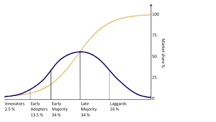
Nearly as important as price, income is also examined due to its relevance in the adoption
process. Meade and Islam note that ‘heterogeneity of income distribution has been cited by
several authors as the driver of the S shape’ famously associated with Roger’s diffusion of
innovation theory. In brief, Roger’s theory espouses that the adoption process is successively
made up of groups of adopters (Figure 4). The adoption groups typically have similar socio-
economic characteristics and behavioral/risk characteristics within group, but are heterogeneous
between groups. The earlier groups of adopters, such as the Innovators, typically have higher
disposable incomes, higher education, and higher risk tolerance than later groups of adopters. As
a result, it is possible for an innovation to never reach full market saturation if the benefits do not
outweigh the risks for the later groups. The most commonly cited reason for failure of market
adoption progress is inadequate price decline (Golder and Tellis 2004).
©2014 ACEEE Summer Study on Energy Efficiency in Buildings 9-187Additionally, CFL diffusion parameters associated with the adoption of innovation and
the S curve shape may provide some insights into LED adoption. Golder and Tellis (2004) and
Lund (2009) estimate take-off periods for several products ranging from consumer durables to
electronics. Peres et al. contends that take-off is a result of price reductions, which in turn
reduces consumer risk. This explains why take-off is much longer for durable goods, 35 – 45
years, as opposed to less expensive White Goods (appliances and housewares), whose take-off
ranges from 6 – 23 years. Brown Goods (leisure goods and electronics) had the lowest take-off
time period ranging from 2 – 17 years. Lighting is not considered part of the Brown Good or
‘status enhancing’ goods. Instead, lighting is considered more of a houseware, and could expect
similar take-off time periods.
Figure 4. Adopter groups according to Roger’s Diffusion of Innovation
theory. Source: Roger’s 1995.
Another aspect of diffusion research which may provide analytical insights into new
lighting products are the coefficient of imitation and the coefficient of innovation, two
parameters of the Bass model (Bass 1969). The coefficient of imitation accounts for internal
influences or ‘word of mouth’ effects, while the coefficient of innovation is widely viewed as the
effect of external or advertising effects. These coefficients influence the shape of the curve. The
coefficient of innovation has a greater impact on the front end of the curve. A purely innovative
diffusion curve creates a more aggressive exponential shape. Alternatively, a more imitative
process creates the S curve shape. The coefficient of imitation is always higher than the
coefficient of innovation, hence the pervasiveness of the S shape. Review articles on diffusion
on innovation by Kohli, Lehmann, and Pae (1999) and Chandrasekaran and Tellis (2007) provide
the following ranges for the diffusion parameters:
©2014 ACEEE Summer Study on Energy Efficiency in Buildings 9-188Table 3. Value ranges for coefficient of innovation and imitation from review of
more than 200 products. Source: Kohli, Lehmann, and Pae 1999 and
Chandrasekaran and Tellis 2007
0.38 – 0.53 Chandrasekaran and Tellis
Coefficient of Imitation
0.23 – 0.34 Kohli et al.
0.0007 – 0.03 Chandrasekaran and Tellis
Coefficient of Innovation
0.0052 – 0.0115 Kohli et al.
One could expect the diffusion parameters for LEDs to be somewhat similar to CFLs.
Relative values of the CFL parameters within the suite of goods listed above may provide
intuition into how a new lighting innovation may adopt. With regard to price/adoption
relationships, Kohli et al. echo the sentiment of Peres et al. They explain that cheaper, less risk
products, such as housewares have relatively higher coefficients of innovation. Since, lighting
falls within the housewares category, it may also be subject to the relative price sensitivity noted
above.
Other measurements of price sensitivity are income elasticity of demand and own-price
elasticity of demand. Income and price elasticities refer to the responsiveness of demand
associated with income change and changes in price, respectively. Elastic goods are price
sensitive and will have an elasticity greater than 1. Inelastic goods have elasticities between 0
and 1. A normal good means an increase in income causes an increase in demand. A normal
good can be income elastic or inelastic. A luxury good means that an increase in income causes
a bigger percentage increase in demand and would therefore have an elasticity greater than one.
Allcott and Taubinsky (2013) found own-price elasticity of demand for CFLs to be very elastic.
Using a test group and incentives equal to 20% of the bulb cost, they estimated CFL price
elasticity to be approximately -1.5.
This paper also examines income and price elasticities of CFLs to use as reference points
for LED adoption1. Next, we examine the CFL market adoption characteristics and some
economic characteristics. Examining these adoption, or diffusion characteristics will help
explain how many years it took for the market to ‘take-off’, when it hit its maximum penetration
rate, and provide estimates of its total penetration, or cumulative sales volume. It is well known
that the cumulative sales of many new innovations follow an adoption path that is sigmoidal or S
shaped based on Roger’s theory of diffusion. One of the most prolifically used models which
captures this shape is the Bass (1969) model. Therefore, this paper uses the Bass model to
estimate the coefficients of imitation and innovation for CFLs to see what may be in store for
LEDs. Lastly, this paper estimates a future price trajectory of LEDs based on the existing price
trend to draw some inferences about LEDs ability to saturate the market.
Methodology
As mentioned in the introduction, the focus of this paper is on the adoption characteristics
of CFLs as a means to glean insights into possible adoption paths for LEDs. Although both sales
and price data are available for CFLs, sales data was unobtainable for LEDs. An LED price
series was created through actual and interpolated data. LED prices were sporadically available
1
Due to declining investment in halogen R&D, along with increasing efficacy standards of EISA’s phase 2,
halogens are not part of the analysis.
©2014 ACEEE Summer Study on Energy Efficiency in Buildings 9-189from LEDinside (2010 – 2014). More specifically, monthly prices for sales weighted averages
of 40w and 60w LEDs in the US market were taken from LEDinside’s online articles. Also,
approximately, 30% of the monthly values were missing, in which case prices were estimated via
logarithmic interpolation. Further, if monthly shelf survey data was available by CLEAResult
(2012 and 2013), this data was used for any missing values. There were some minor
discrepancies between U.S. average prices and regional prices in the Pacific Northwest, however,
the overall data trend looked reasonable (Figure 1). LED forecasted prices are estimated based
on the logarithmic trend produced in Figure 1 and expressed in Equation 1.
Pt = -7.777ln(t) + 49.024 (1)
where P is price at time t. It is the first cost comparison of the LED price forecast with CFLs that
will provide insights into the potential success of LEDs. Annual general purpose CFL prices
were taken from annual shelf surveys conducted by KEMA DNV as part of NEEA’s CFL
initiative.
In addition to price analysis, we examine some CFL adoption characteristics using the
following Bass estimation:
Ү(t) = m[(1-e-(p+q)t)/(1 + (q/p)e-(p+q)t)] (2)
where, Y(t) denotes cumulative adoptions at time t, m is the market size, p is the coefficient of
innovation, q is the coefficient of imitation, and e is the exponential function. For a full
derivation of equation 1 refer to Bass (1969). Adoptions are gross sales of CFLs in the Pacific
Northwest, including sales that are used for replacements. A nonlinear estimation technique is
used to derive the parameters.
We also want to examine income and own-price elasticity. Ideally, one would want to
control for underlying sales dynamics resulting from diffusion (Tellis 1988; Parker 1992) with
functional forms suggested by Jain and Rao (1990). However, the limited number of
observations does not allow for the inclusion of the explanatory variables, income and CFL
price, in Eq 2. Another consideration is that autocorrelation is common in time series, so a
simple autoregressive model (AR1) corrected for first order autocorrelated errors is used to
estimate elasticities with the following function
Ү(t) = ln(Хt) β + μt , (3)
μt = ρμt-1 + ԑ (4)
where β’s and ρ are coefficients, and Хt = x1, x2 represent logged price and logged income.
Prices reflect general purpose, medium screw-based CFLs (DNV KEMA 2013). Income reflects
population weighted average state income for Washington, Oregon, Idaho, and Montana. All
models were estimated using the software package, Regression of Time Series Analysis by
Estima 2010.
©2014 ACEEE Summer Study on Energy Efficiency in Buildings 9-190Results
As expected, there were not enough observations to get the Bass model to converge while
including the independent variables, income and price. However, the simplified Bass model
provided a reasonable fit of the data. Graphs of the annual and cumulative actual data, and their
Bass prediction curves (Figures A1 and A2), followed by the estimation results are provided in
the appendix (Table A1). The coefficient of innovation for CFLs is 0.001, falls within the
coefficient range supplied by Chandrasekaran and Tellis, but below the range of surveyed good
analyzed by Kohli et al. in Table 2. This may be due to the relatively high price of CFLs
compared to incandescent bulbs, as well as the degree of their ‘innovativeness’, ie. the bulbs look
quite different from incandescent bulbs and are perceived to not perform as well (DNV KEMA
2013). Conversely, the coefficient of imitation is relatively high at 0.48 suggesting most of the
growth in sales occurred in the latter stages of the CFL life cycle. Correspondingly, the period of
most rapid growth occurred in 2006, nine years after marketing efforts began. Additionally,
CFLs reached a maximum market saturation rate of 33% in 2008. Although it is expected that
bulb sales will decline as sockets are filled with more efficient bulbs, the fact remains that CFL
socket saturation only reached 24% suggesting that the latter adoptive groups were never
reached.
In addition to the diffusion parameters, income and own-price elasticities were also
calculated. The first equation estimated was a simple log linear model, however, the errors
presented autocorrelation, as predicted. The estimation was then run using an AR(1) model, as
defined by Equations (3) and (4) in the methodology, of logged price and income on logged sales
(Table A2). This estimation was challenged given a usable observations limit of 16. However,
the results of this model gives reasonable results, i.e. realistic coefficient values, correct signs,
and reasonable significance given the limited data. It is most likely that collinearity exists. Due
to limited data the model is unable to distinguish between price and income effects as evidenced
by a high R2 of 0.89 when logged income is regressed on logged price (not shown in the
Appendix). As a result, individual AR(1) regressions of price and income against sales were
used to provide elasticity relationships (Tables A3 and A4). Elasticity results from all three
regressions provide a range of elasticities. The own-price elasticity ranges from -0.94 to -2.99
indicating strong price sensitivity. Income elasticity ranges from 6.10 to 7.80 strongly indicating
that CFLs are a luxury good.
Lastly, estimated LED prices using the existing price trend, indicates that average annual
price per bulb may drop to $11.50 by the year 2020 (Figure 5). Assuming that the CFL price
trajectory will also follow its historic path, future CFL price will hover around $4.00, making
LEDs 2 to 3 times more expensive by the year 2020. This LED estimate may be high. IHS
forecasts an average of $12.70 per bulb in 2014, much lower than the extrapolated average of
$18.24. Further, Huston contends that a LED “price war” will erupt in 2014 possibly driving
prices downward at a rate exceeding the forecasted trend.
Conclusions
For long-run adoption success, the question is ‘can the benefits of long-run savings
outweigh the barrier of first cost?’ To examine this question, the adoption characteristics of
CFLs are examined. The Bass model estimation suggests that CFLs are in a decline phase
despite the advent of EISA. Often cited reasons for the decline are quality concerns and the
©2014 ACEEE Summer Study on Energy Efficiency in Buildings 9-191availability of cheap substitutes such as halogens bulbs. Although to a much lesser extent, LEDs
seem to have some of similar quality issues that have nagged CFLs (Green American 2010;
AZCentral.com 2014). However, Philips, Osram, GE and other major manufacturers seem
highly motivated given price their price incentives. Additionally, utilities will start to provide
significant rebates which will reduce the price even further. Some believe that LEDs will
eventually replace all incandescent bulbs with CFLs only a temporary solution. Nonetheless, the
results of this research suggest that in the lighting market, CFL bulbs are highly income and
price elastic. It is the belief of this researcher that LEDs may be subject to similar price
sensitivity. Time will tell consumers how consumers will weigh the non-financial benefits of the
LEDs over LED first cost.
Figure 5. Actual and projected LED average prices for 40 watt and 60 watt equivalents.
Source: Holland, 2014.
References
Allcott, H. and D. Taubinsky. 2013. “The Lightbulb Paradox: Using Behavioral Economics for
Policy Evaluation.” New York Univeristy Working Paper.
AZCentral.com. January 2014. “Despite cost, LED lights are better than CFLs.”
http://www.azcentral.com/home/articles/20130403led-lights-better-cfls-reasons.html
Bass, F. 1969. “A new product growth model for consumer durables.” Management Science 15:
215-227.
Bonn, L. 2012. “A Tale of Two CFL Markets: An Untapped Channel and the Revitalization of
an Existing One.” ACEEE Summer Study on Energy Efficiency in Buildings.
http://www.aceee.org/files/proceedings/2012/data/papers/0193-000197.pdf
Calem, R. December 2013. “2014 Incandescent Bulb Ban: Here are your alternatives.”
http://www.tomsguide.com/us/light-bulb-guide-2014,review-1986.html
©2014 ACEEE Summer Study on Energy Efficiency in Buildings 9-192Chandrasekaran, D. and G. Tellis. 2007. “A Critical Review of Marketing Research on Diffusion
of New Products.” Marshall School of Business Working Paper No. MKT 01-08, pp. 39-80.
CLEAResult, formerly Fluid Marketing, Inc. Correspondence June 2012 and June 2013.
Department of Energy (DOE), EERE. US Lighting Market Characterization. Volume 1.
September 2002, prepared by Navigant Consulting, Inc.
Department of Energy (DOE), EERE. 2010 US Lighting Market Characterization. January
2012, prepared by Navigant Consutling, Inc.
DNV KEMA Energy and Sustainability. July 2013. 2012 – 2013 Northwest Residential
Lighting Market Tracking Study. Prepared for Northwest Energy Efficiency Alliance.
Eartheasy.com. “Energy Efficient Lighting.” http://eartheasy.com/live_energyeff_lighting.htm,
March 2014.
Ecotope. 2012. Residential Building Stock Assessment: Single Family Characteristics and
Energy Use. Prepared for Northwest Energy Efficiency Alliance, October 2012.
Energy Independence and Security Act of 2007. H.R. 6 (110th). January 12, 2007.
Estima. Regression Analysis of Time Series (RATS). Version 8. Evanston, Il. 2010.
Golder, P. and G. Tellis. 2004. “Growing, growing, gone: Cascades, diffusion, and turning
points in product life cycle.” Marketing Science, 23(2): 207-218.
Green America. 2010. “CFLs vs LEDs.” http://www.greenamerica.org/livinggreen/CFLs.cfm
Huston, R. “Will 2014 Be the Year of the $10 (60 Watt Equivalent) LED Bulb?” PRWeb.
September 20, 2013. http://www.prweb.com/releases/2013/9/prweb11144359.htm
Jain, D. and R. Rao. “Effect of Price on the Demand for Consumer Durables: Modeling,
Estimation, and Finding.” Journal of Business & Economic Statistics, 8:163-170.
Kim, C., R. O’Conner, K. Bodden, S. Hockman, W. Liang, S. Pauker, and S. Zimmermann all of
WSGR. May 2012. Innovations and Opportunities in Energy Efficiency Finance. White
Paper. http://www.wsgr.com/publications/PDFSearch/WSGR-EE-Finance-White-Paper.pdf
Kohli, R., D. Lehmann, and J. Pae. 1999. “Extent and impact of incubation tie in new product
diffusion.” Journal of Product Innovation Management, 16:134-1444.
LaBlanc, G. “Motivating Behavioral Change: Lessons from Behavioral Finance.” Keynote
Speaker, Efficiency Exchange 2014. https://conduitnw.org/Pages/Article.aspx?rid=484
LEDinside of TrendForce Corp. http://ledinside.com/ . Numerous web links between March
2010 and January 2014.
©2014 ACEEE Summer Study on Energy Efficiency in Buildings 9-193Lightbulbchoice.com, 2014. “The law – Energy Independence and Security Act (EISA) of
2007.” http://lightbulbchoice.com/the-law/
Lighting.Com, 2014. http://lighting.com/doe-forecast-leds-74/.
Lund, P. 2006. “Market Penetration Rates of New Energy Technologies.” Energy Policy,
34:3317 – 3326.
Meade, N., and T. Islam. 2006. “Modeling and forecasting the diffusion of innovation – A 25-
year review.” International Journal of Forecasting, 22: 519-545.
Navigant Consulting, Inc. and SAIC. June 2013. “Technology Forecast Updates – Residential
and Commercial Building Technologies – Reference Case.” Prepared for the U.S. EIA.
http://www.eia.gov/analysis/studies/buildings/equipcosts/pdf/appendix-c.pdf
Parker, P. 1992. “Price elasticity dynamics over the adoption life cycle.” Journal of Marketing
Research, 29(8): 358-367.
Peres, R., E. Muller, and V. Mahajan. 2010. “Innovation diffusion and new product growth
models: A critical review and research directions.” International Journal of Research in
Marketing, 27: 91-106.
Rogers, E. “Diffusion of Innovations.” New York: Free Press, 1995.
Tellis, G. “The Price Elasticity of Selective Demand: A Meta-Analysis of Econometric Models
of Sales.” Journal of Marketing Research, 25 (11): 331-341.
The Verge. October 2013. http://www.theverge.com/2013/10/3/4798602/walmart-gets-
aggressive-on-lef-bulb-pricing/
Appendix
CFL Actual vs Predicted Sales
22500000
Actual
20000000 Predicted
17500000
15000000
12500000
10000000
7500000
5000000
2500000
0
1997 1998 1999 2000 2001 2002 2003 2004 2005 2006 2007 2008 2009 2010 2011 2012
Figure A1. Annual CFL sales versus estimated annual sales produced by a simple Bass model.
©2014 ACEEE Summer Study on Energy Efficiency in Buildings 9-194CFL Actual vs Predicted Cumulative Sales
140000000
Actual
Predicted
120000000
100000000
80000000
60000000
40000000
20000000
0
1997 1998 1999 2000 2001 2002 2003 2004 2005 2006 2007 2008 2009 2010 2011 2012
Figure A2. Cumulative CFL sales versus estimated cumulative sales produced by a simple Bass model.
Table A1. Results from bass model estimation
Nonlinear Least Squares - Estimation by Gauss-Newton
Dependent Variable SALES ; Annual Data From 1997:01 To 2012:01
Centered R^2 0.90112; ; Uncentered R^2 0.96117
Mean of Dependent Variable 8044928.375 ; Std Error of Dependent Variable 6680220.6536
Standard Error of Estimate 2256368.578 ; Sum of Squared Residuals 6.6185e+013
Log Likelihood -255.1102 ; Durbin-Watson Statistic 1.5864
Variable Coeff Std Error T-Stat Signif
1. P 0.489063 0.054508 8.97233 0.00000062
2. Q 0.001334 0.000685 1.94630 0.07355930
3. M 144658398.318 11822539.005 12.235 0.00000002
Table A2. Results from autoregressive model of logged price and income on logged sales.
Regression with AR1 - Estimation by Beach-MacKinnon
Dependent Variable LNSALES ; Annual Data From 1997:01 To 2012:01
Centered R^2 0.94813 ; Uncentered R^2 0.99941
Mean of Dependent Variable 15.15182 ; Std Error of Dependent Variable 1.67517
Standard Error of Estimate 0.44551 ; Sum of Squared Residuals 2.18331
Log Likelihood -7.1040 ; Durbin-Watson Statistic 1.19950
Variable Coeff Std Error T-Stat Signif
1. Constant -47.05411576 26.25260737 -1.79236 0.10058941
2. LNINCOME 6.10350494 2.41790436 2.52430 0.02825876
3. LNPRICE -0.94540904 0.77473377 -1.22030 0.24786567
4. DUM2001 1.16199221 0.37149532 3.12788 0.00961396
5. RHO 0.69875280 0.31200375 2.23957 0.04673684
Table A3. Results from autoregressive model of logged income on logged sales
Regression with AR1 - Estimation by Beach-MacKinnon
Dependent Variable LNSALES ; Annual Data From 1997:01 To 2012:01
Centered R^2 0.94303 ; Uncentered R^2 0.9993546
Mean of Dependent Variable 15.15182 ; Std Error of Dependent Variable 1.67517
Standard Error of Estimate 0.44700 ; Sum of Squared Residuals 2.39772
Log Likelihood -8.0044 ; Durbin-Watson Statistic 1.0210
Variable Coeff Std Error T-Stat Signif
1. Constant -66.48776223 18.43731957 -3.60615 0.00360499
2. LNINCOME 7.80585242 1.76956319 4.41117 0.00084861
3. DUM2001 1.23892110 0.35127181 3.52696 0.00416969
4. RHO 0.78845864 0.18958101 4.15895 0.00132526
©2014 ACEEE Summer Study on Energy Efficiency in Buildings 9-195Table A4. Results from autoregressive model of logged price on logged sales
Regression with AR1 - Estimation by Beach-MacKinnon
Dependent Variable LNSALES ;Annual Data From 1997:01 To 2012:01
Centered R^2 0.91700 ; R-Bar^2 0.89625 ; Uncentered R^2 0.99905
Mean of Dependent Variable 15.15182 ; Std Error of Dependent Variable 1.67517
Standard Error of Estimate 0.53957 ; Sum of Squared Residuals 3.49365
Log Likelihood -10.6238 ; Durbin-Watson Statistic 1.7471
Variable Coeff Std Error T-Stat Signif
1. Constant 20.19694647 0.75746749 26.66378 0.00000000
2. LNPRICE -2.99927162 0.41945411 -7.15042 0.00001164
3. DUM2001 1.13952822 0.50292272 2.26581 0.04276009
4. RHO 0.41385777 0.31759338 1.30311 0.21698845
©2014 ACEEE Summer Study on Energy Efficiency in Buildings 9-196You can also read