Analyzing Student Performance with Personalized Study Path and Learning Trouble Ratio
←
→
Page content transcription
If your browser does not render page correctly, please read the page content below
Analyzing Student Performance with Personalized Study
                Path and Learning Trouble Ratio

                            James Shing Chun Yip                   Raymond Chi-Wing Wong
                                   The Hong Kong University of Science and Technology
                                             {scyipaa, raywong}@cse.ust.hk

ABSTRACT                                                           concepts throughout a course.
Massive Online Open Courses (MOOCs) have become very
popular nowadays and are attracting a lot of attention from        As a clear learning path enables both instructors and stu-
both learners and researchers. Learners benefit from their         dents to improve learning efficiency. This motivates us to
availability of learning materials such as lecture notes, videos   visualize the learning path in a clear and simple way. In
and self-tests. However, most MOOCs are a one-size-fit-all         this paper, we introduce a method of visualizing an ordered
model and does not meet the individual needs of learners.          learning graph to represent the order of the learning path.
For example, each learner is shown a “pre-defined” order of        In our graph, it contains learning concepts of a course that
study for each different learning concept in a course. It is ob-   link together with a number which we call learning trou-
served that different learners have different learning paces,      ble ratio showing the strength of dependency as well as a
and how good a learner understands one learning concept is         weight. This ratio indicates the difficulty of such a pair of
heavily dependent on how good s/he understands the pre-            concepts for the students to study. It also emphasizes the
requisite of this learning concept (which is also a learning       concepts both students and instructors should pay attention
concept). Motivated by this, some researchers would like to        to. Not only that, the ratios for each pair can be dynami-
propose some personalized suggestions for each learner so          cally updated by using students’ learning performance and
that they could learn certain concepts in different order. In      the learning graph.
this paper, we introduce a method for visualizing an order-
ing of learning concepts concisely and showing how strongly        We choose the course “COMP102X Introduction of Java
one learning concept is related to another learning concept.       Programming” with a duration of 14 weeks offered by HKUST
                                                                   on Open edX. The course is administered by Professor T.C.
                                                                   PONG since June 2014, as a basis for developing our sys-
Keywords                                                           tem and also an extension of a course on Open edX platform.
Learning Analytics, Visualization, Educational Data Mining         This course is composed of 12 concepts with 91 questions.
                                                                   10564 unique students, with at least one record of question
1.    INTRODUCTION                                                 submission, enrolled in the course. A demonstration (https:
Most courses in MOOCs are used to present their curricu-           //www.youtube.com/watch?v=KdxVHWSMNi4) and source cod-
lum in a chapter-by-chapter format. For example, it can be a       es (https://github.com/shingyipcheung/study-path-bac
list of videos with lecture notes for each chapter in an online    kend) are available. In this paper, our contributions can
platform like Coursera. This design is linear (or predefined)      be summarized as: We proposed a method of visualizing a
and insufficient for emphasizing the relationships between         learning graph which can be “weighted” and “ordered”; We
chapters or concepts. In contrast, our knowledge should            use the data from an existing MOOC to recommend the
be based on prerequisites and even the prerequisites of pre-       learning paths to students with the compact visualization;
requisites. These relationships recursively form a learning        We make use of modern web frameworks and open source
graph where each node corresponds to a learning concept.           libraries to implement the system that is available online;
Then an edge from one node to another node correspond-             We provide examples to suggest actions for instructors and
ing to that one learning concept is a prerequisite of another      students based on the visualization.
learning concept. This graph is actually a directed acyclic
graph (DAG) which is able to generate many topological             The remainder of this paper is summarized as follows: In
order paths. Note that there are many ways to study all            Section 2 and Section 3 we introduce related works and
                                                                   the problem we are focusing on. In Section 4 we explain
                                                                   our methods in details from collection to generate Learn-
                                                                   ing Trouble Ratio and Personalized Path. In Section 5, we
                                                                   demonstrate how to use modern frameworks and libraries
                                                                   to implement the visualization. Finally, we suggest some
                                                                   cases to help the instructor to identify students who are in
                                                                   “trouble” in Section 6, and conclude in Section 7.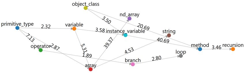
Figure 1: Default ordered learning graph of COMP102X Introduction of Java Programming

2.   RELATED WORK                                                 including the demographic info of students. Although their
The task of prerequisite relation, to predict whether a con-      visualizations aid the instructor to see the overall picture in
cept or skill is a prerequisite of another, has been studied      different kinds of data, it might be too low-level for students
by different approaches. The data are mostly collected from       to understand what is being presented to them. In contrast,
Wikipedia. In [[3], [13], [9]], semantic and video features       we try to use the learning graph with suggested study path-
are designed to compare the relatedness between concepts,         ways to point out which concepts should be learned earlier.
and predict the relations by the supervised classification ap-
proach. Liang [10] et al. proposed an objective function          Grosse and Reed [6] created a web application Metacademy
as a soft margin SVM where each course is represented by          for autodidacts to learn science subjects with the help of
the term frequency-inverse document frequency (tfidf) to re-      a learning (concept) graph. Their work is very similar to
cover the strength of prerequisite relations. Adjei et al. [1]    ours but without the education data provided by MOOC.
developed a system to stress the problematic links in a pre-      Further, the application only contains a single learning path
requisite skill structure where they used linear regression to    handcrafted by the creators for learners to follow. Compared
find the strength as the coefficients in the equation. Our ap-    with their application, our work has two major advantages
proach is relatively simpler and more intuitive, we use the       which could not be found in their studies. First, we combine
assessment results to measure the “troublesome” of the rela-      the learning graph structure and MOOC data to provide
tions by the probability ratio. This measurement also points      strength among the concepts - learning trouble ratio which
out some pairs may create problems for students.                  emphasizes the correlations that students should pay atten-
                                                                  tion to. Second, we provide multiple learning paths which
For visualizing graphs, previous studies have developed dif-      are in topological orders. Our graph can be transformed in
ferent tools for various applications. North [11] created a       an ordered way to represent one of the paths.
visual debugger called dotty which can provide an interac-
tive operation for users. Another paper proposed a visual-
ization method for Extract Method refactoring which is for        3.   PROBLEM DESCRIPTION
moving a part of the original code to a separate new method       We are given a learning graph containing nodes which cor-
in the form of the program dependency graph [7]. A node           respond to a learning concept and edges corresponding to
on the graph is defined as a line of code, and an edge indi-      the correlation between two learning concepts. Specifically,
cates a reference or a definition of a variable. Their work       we represent a relationship between two (learning) concepts
aims to identify any potential nodes that can be refactored       with a dependency. A concept could be dependent on one or
without using big data, whereas in our work the goodness          more concepts. For example, in Figure 1 (showing the rela-
assessments of each node are data-driven. In this paper, we       tionship of learning concepts in a Java programming course),
focus on visualizing the learning dependency graph contain-       we learn primitive_type first and then operator since op-
ing concepts as nodes which could be helpful for science and      erator depends on primitive_type. We use a directed
engineering subjects because of the high correlation among        graph to represent all dependencies among all concepts in
the concepts.                                                     a course. In general, each node in a graph is a learning con-
                                                                  cept. In layman’s terms, the graph is a representation of the
After MOOCs became popular, more studies emerged on vi-           prerequisites of concepts. The graph is always sparse since
sualizing educational data. Qu and Chen [15] pointed out          there are not many dependencies from one to other learning
that education stakeholders will benefit from the intuitive       concepts. Therefore, we use an adjacency list to represent
visualization to reduce the learning curve. Shi et al. [16] de-   the directed graph. Figure 1 shows the learning graph of
veloped a system which contains several views to aid learn-       the course COMP102X in Open edX offered by Prof. T. C.
ing analytics by using clickstream data from Open edX. For        Pong drawn by D3.js [2].
example, their demonstration provides the graph of a course
                                                                  In this paper, we study two problems. The first problem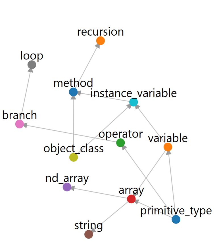
(b) Drawing from left to right

     (a) Initialized with random positions

                                             Figure 2: Learning graphs with crossed edges

is to recommend a personalized study path to each student                         Concept           Question id   Weight
based on the dependency graph. The second problem is to                        primitive_type          Q1          1.0
visualize the personalized study path of each student in a                     primitive_type          Q2          1.0
concise way.                                                                   primitive_type          Q3          0.8
                                                                               primitive_type          Q4          1.0
In this paper, we plan to show the study path as seen in                          variable             Q5          1.0
Figure 1 such that the first learning node in the order is                        variable             Q6          1.0
shown in the leftmost place in the graph, the second learning                     variable             Q4          0.6
node is shown in the second leftmost place, and so on.
                                                                     Table 1: Example. Mapping of Concepts to Questions with
However, how to visualize the study path concisely is a chal-        weights
lenge. In Figure 1, we could observe that no edges cross each
other. Due to personalization, different nodes may appear in
different positions in the graph. Without “careful” design, it       According to Open edX documentation, the students’ learn-
is “possible” that one edge may cross another edge. For ex-          ing progress data are stored on the table
ample, if the node operator in Figure 1 is moved to a place          courseware_studentmodule. This table holds the most re-
under the (virtual) horizontal line passing through the node         cent course state, including the most recent problem sub-
variable, the edge between variable and array will cross             mission and unit visited in each subsection. We can retrieve
with the edge between the primitive_type and operator.               information about who answered which question and also
Drawing directed graphs in a clear way requires different            the obtained score.
settings such as node positions given the graph structure.
Figure 2 shows graphs without any adjustments to the node            Specifically, we retrieved the score of each question of each
positions which looks very unclear.                                  student by 5 fields (module_type, module_id, student_id,
                                                                     grade, and max_grade). module_id is the key for each prob-
                                                                     lem. We only consider module_type with value problem.
4.     METHODOLOGIES                                                 The term max_grade might be confusing since it denotes the
In this section, we propose how to generate the learning             number of sub-problems for a problem. The relative score
trouble ratios and personalized study paths from the student         of a problem is between 0 and 1.
performance and the dependency graph. First, we take the
course COMP102X as an example to formulate the score cal-
culation in Section 4.1. Next, we use the scores under such           4.1.2    Problem Weighting
a pair of concepts to quantify its correlation in Section 4.2.       Instructors could set the weight to a problem for a learning
The remainder of this part explains the algorithm to gen-            concept. Specifically, each problem is mapped to one learn-
erate all topological arrangements given a learning graph in         ing concept or more. Each learning concept is mapped with
Section 4.3. A fitness function is designed to measure which         at least two questions. An example in Table 1 shows there
arrangements fit a student. We also describe how to visual-          are 4 problems in primitive_type with weights between 0.8
ize the directed graph that minimizes the number of crossed          to 1. The problem with id “Q4” is mapped to both primi-
edges in Section 4.4.                                                tive_type and variable.

4.1      Learning Performance                                         4.1.3    Student Score Calculation
                                                                     With the problem weight mapping and the progress table
4.1.1      Student Performance Collection                            from the previous two sections, we use the following formula
to calculate the scores of all students. if the numerator is larger than the denominator, we can
infer that it is more likely that a student will have trouble
when studying the concept. The higher the ratio, the more
X gradep important it is that the prerequisite should be paid attention
scoreconcept = wp · (1) to.
p∈concept
max gradep
For simplicity, we divide students into 4 groups in Table 3
where wp is the pre-defined weight of the problem p, gradep where each group can easily be found by database query.
and max gradep are the field values in Section 4.1. The ratio is calculated by set operations. For example,
Sprev,below denotes the set of students who are below av-
Each score of a concept is scaled by min-max normalization. erage in the preceding concept Cprev .
Therefore, all scores of the concepts of a student in a course
are found. pair
Cprev Cnext
Below Sprev,below Snext,below
scorecourse = {normalize(scoreconcept )|concept ∈ course} Above Sprev,above Snext,above
(2)
Table 3: Four sets of students
By this calculation, we found 10564 unique students with at
least one score (some of them dropped out) in COMP102X.
The mean scores are summarized in Table 2.
concept mean Learning trouble ratio
array 0.712297 |Sprev,below ∩Snext,below |
branch 0.423561 |Sprev,below ∩Snext,below |+|Sprev,below ∩Snext,above | (4)
=
instance_variable 0.519257 |Snext,below ∩Sprev,above |
|Snext,below ∩Sprev,above |+|Sprev,above ∩Snext,above |
loop 0.521106
method 0.235022
nd_array 0.312867 From Equation 4, we intersect the sets and compute the
object_class 0.542028 risk ratio by the cardinalities. For example, assume we
operator 0.375814 have all the students’ IDs in Snext,below = {2, 3, 4} and
primitive_type 0.315577 Sprev,above = {3, 4, 5}. The number of students who are
recursion 0.748562 above average in Cprev but below average in Cnext , i.e.,
string 0.572801 |Snext,below ∩ Sprev,above | is 2.
variable 0.463743
The ratios can also be imported as the weights for each edge
Table 2: mean concept scores in COMP102X in the graph and can be dynamically updated based on the
students’ performance for an ongoing course (see Figure 1).
4.2 Strength of Correlation Between Learn-
ing Concepts 4.3 Personalized Path Generation
To estimate the strength of the correlation of each pair in Our method is to enumerate all possible topological paths
the dependency graph, we adopt the risk ratio [17] as an based on the given dependency graph G = (V, E) and re-
indicator that we call learning trouble ratio which produces turns the top 10 paths evaluated by some fitness functions.
the ratio of the probability of the performance between two We use the basic backtracking method to generate all pos-
groups. We define that a student whose score is greater than sible arrangements in Algorithm 1. The algorithm begins
or equal to the average in a concept as “Above-Average”, with initializing all vertices as not visited. It then adds the
otherwise they are “Below-Average”. In this paper, the av- vertex which is not visited and is of indegree 0 to the result
erage score is equivalent to the mean score, the median may followed by removing all edges pointing from that vertex.
also be applied. There are “Above-Average” and “Below- Lastly, it calls itself recursively and backtracks. Another
Average” groups for each concept. We define a pair of con- efficient algorithm [8] can also be applied.
cepts (Cprev , Cnext ) in the learning graph where Cprev is
the prerequisite of Cnext . The numerator on Equation 3 is The fitness functions can be designed for different purposes.
interpreted as the probability of a student whose result of One fitness function we used is the ratio relative to the mean
concept Cnext is “Below-Average” given that the result of score. A concept should be learnt first because the score of
concept Cprev is “Below-Average” as well. the student in that concept is far from being an average
student.
|V |
X 1 scoremean (p[i]) − scoret (p[i])
P (Cnext,below |Cprev,below ) f it(p, t) = (5)
Learning trouble ratio = (3) i scoremean (p[i])
P (Cnext,below |Cprev,above ) i=1
The above equation evaluates a path p for a student t, where
Students can be below average in a certain concept, however, scoremean (·) denotes the mean score of the concept in thecourse globally, and scoret (·) denotes the score of the stu- weight, and δ(v, u) is the minimum length constraint input
dent t in that concept. For example, given two paths. by users.
array → branch
X
minimize w(v, u)(λ(u) − λ(v))
branch → array
(v,u)∈E (6)
A student whose score in array and branch are 0.6 and 0.5 subject to λ(u) − λ(v) ≥ δ(v, u), ∀(v, u) ∈ E
respectively. From Table 2, we see that the mean score of
array and branch are about 0.7 and 0.4 respectively. The
first path gives the fitness = 11 0.1 + 21 −0.1 ≈ 0.05952, while Two nodes with the same rank will have the same x-coordinate
0.7 0.6
1 −0.1 1 0.1 if the drawing is from left to right. Next, it uses a heuristic
the second path gives 1 0.6 + 2 0.7 ≈ −0.09523. There-
approach that iteratively finds the coordinates to minimize
fore, the first path should be given higher priority than the
the number of crossed edges of the ranked graph until reach-
recommendation.
ing the maximum number of iterations. This algorithm has
been implemented by Dagre [14]. The final graph shows a
Algorithm 1 All Topological Orders
clear layout of the input order without crossing edges (see
Input: a directed graph G = (V, E) Figure 4 in contrast to Figure 2).
Output: a list of paths P in different orders
1: procedure Topological All(V, E) 5. IMPLEMENTATION
2: S←∅ . A set to store nodes are not visited The system is built using two Web frameworks, Django and
3: P ← empty . A list to store result paths Vue.js, for backend and frontend, respectively. Django pro-
4: p ← empty . A temporary path vides us with powerful Python libraries such as Numpy and
5: for each v ∈ V do Pandas for data processing that help to build a web applica-
6: indegree[v] ← 0 tion. The web interface also utilizes D3.js for visualization.
7: insert v into S
8: for each (u, v) ∈ E do Our method has been employed on the system that can gen-
9: indegree[v] ← indegree[v] + 1 erate personalized topological order paths. First, we apply a
10: Topological Recursive(V, E, S, P, p) diversified path algorithm to select the most representative
11: return P paths [4]. These paths are static to all students. To make
12: procedure Topological Recursive(V, E, S, P, p) them personalized, we use some fitness functions to enhance
13: if S is empty then the result. For example, one fitness function is based on
14: insert p into P performance. If the student’s result is not good, the related
15: else concepts should be given a higher weighting. Finally, the
16: for each v ∈ V do pipeline produces the best 10 paths as a result.
17: if v ∈ S and indegree[v] = 0 then
18: for each u such that (v, u) ∈ E do
19: indegree[u] = indegree[u] − 1
20: push v into p
21: remove v from S
22: Topological Recursive(V, E, S, P, p) Figure 3: Flow of generating 10 personalized paths
23: insert v into S
24: pop the last element from p
25: for each u such that (v, u) ∈ E do
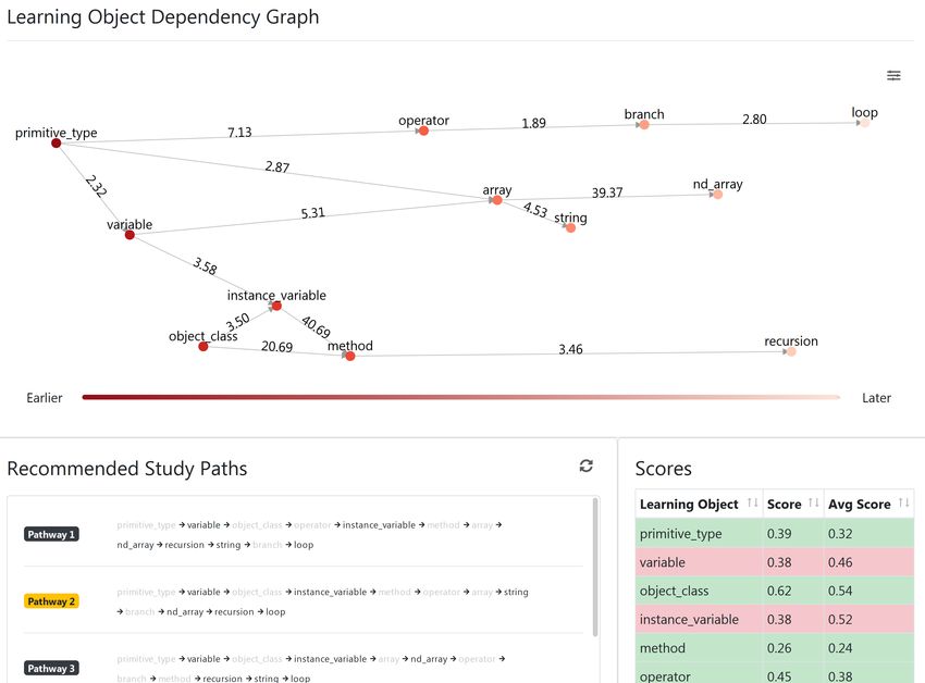
The system has a component called “Recommended Study
26: indegree[u] = indegree[u] + 1
Paths” showing the 10 “best” paths, which are recommended
based on the performance of learning concepts of a student
and the dependency strength among the learning concepts.
4.4 Visualizing Learning Graph Each of this path is shown in two formats. The first format
To draw the learning graph, we employ the web visualization has a sequential order as shown at the bottom part of Fig-
framework D3.js [2]. The force simulation module in D3 is a ure 4 (which shows 2 paths, namely Pathway 1 and Pathway
common feature of visualizing graphs. The module provides 2). The second format is a graph format where the leftmost
multiple forces in the simulation. For example, the centering node in the graph corresponds to the earliest learning con-
force for positioning the nodes at the center of the visual cept to be learnt and so on. One path in the second format
space while the “collision” force adds a force to each node could be found at the top part of Figure 4 (which shows the
with a given radius as a repulsive force to prevent nodes from second format of Pathway 2).
being close to each other. However, D3 itself does not handle
the crossed edge problem because using the collision force
alone is insufficient. To address the problem, we first fix the
6. EXPERIMENT
In this section, our goal is to highlight the importance of
x-coordinates of all nodes from left to right with the input
each component including the learning dependency graph
order. At this time, there are many crossed edges. Next, we
with learning trouble ratios, and the learning pathway.
adopt an algorithm [5] for drawing directed graphs. It first
finds the optimal rank assignments λ(v) for each node v by
solving the integer program in Equation 6 where λ(u) − λ(v) 6.1 Learning Dependency Graph and Learn-
represents the length between node v and u, w(v, u) is the ing Trouble Ratio(Cprev , Cnext ) |Sprev,below ∩ |Sprev,below ∩ |Snext,below ∩ |Sprev,above ∩ Learning Trouble Ratio
Snext,below | Snext,above | Sprev,above | Snext,above |
(primitive_type, operator) 1097 1811 115 2059 7.1
(primitive_type, array) 525 101 554 1342 2.9
(primitive_type, variable) 2523 94 888 1252 2.3
(operator, branch) 1206 72 1915 1914 1.9
(branch, loop) 893 68 639 1286 2.8
(array, nd_array) 555 520 19 1430 39.4
(array, string) 718 62 294 1154 4.5
(variable, array) 766 279 184 1149 5.3
(variable, instance_variable) 1123 514 256 1081 3.6
(object_class, instance_variable) 1024 125 514 1507 3.5
(object_class, method) 1343 384 76 1946 20.7
(instance_variable, method) 952 708 23 1609 40.7
(method, recursion) 229 20 410 1134 3.5
Table 4: Learning trouble ratios
Since both the learning dependency graph and the learning concept mean
trouble ratio are presented in the same visualization, they object_class 0.21
are put together as a component. One might think that instance_variable 0.31
we can just make a notice for all students who are below method 0.03
average. However, one major issue in MOOCs is the high array 0.18
dropout rate of learners [12]. Most students treated as bad nd_array 0.15
performers, in our terminology, are “below average” which is
not enough to identify the students who really need helps. Table 5: Mean scores of students who only work on 1 concept
Owing to this, we focus on the students who are at least (None for the others)
making an effort to do some of the exercises but end up
achieving a low score. In short, they are the students who
are “above” in Cprev and “below” in Cnext , i.e., Snext,below ∩
Sprev,above in Equation 4. Since array and nd_array are very dependent (because the
learning trouble ratio between array and nd_array is of
According to Table 4, we can see two pairs (array, nd_array) value 39.37 which is high). Our system provides the par-
and (instance_variable, method) having a high value of ra- allel coordinates plot where users can select multiple score
tio. The trouble ratio not only indicates the strength of ranges to extract the students.
dependency but also makes the target students apparent
among the crowd. Using the dependency graph with the Figure 5 shows parallel coordinates, a lot of “blue” lines
edge values (learning trouble ratios), we can filter out these where each connected line corresponds to a student. It also
students easily, a detailed example is explained in the Case shows a vertical black line for each learning concept. For
Study. example, array has a vertical line denoting the “score” of a
learning concept obtained by a student. If a blue (horizon-
tal) line has a value of 0.8 in the vertical line of array and a
6.2 Learning Path value of 0.2 in the vertical line of nd_array, this means that
Without a suggested learning path, students may randomly the corresponding student (for this blue line) has a score of
pick a concept to study. We expect that this random ap- 0.8 for array and a score of 0.2 for nd_array.
proach would result in a bad performance, especially if a con-
cept has prerequisites the student has not fulfilled. There- In this interface, users could also “highlight” some parts of
fore, we chose 3 (single-length path) pairs of concepts with the vertical lines to select all blue lines out. For example, in
the top 3 highest learning trouble ratio for illustration. Figure 5, we tried to select the students whose score is above
instance_variable → method average in array (shown in the shaded region in the vertical
line of array in the figure) and below average in nd_array
object_class → method (shown in the shaded region in the vertical line of nd_array
array → nd_array in the figure) to check whether there are many such “un-
expected” students (since we expected that students who
We found that students perform badly if they only do the
performed well in array should perform well in nd_array).
exercises for just 1 concept. From Table 5, we see that all 3
pairs: the score of Cnext must be less than the that of the
Finally, we find 19 students (shown in Figure 6). Most stu-
prerequisite Cprev .
dents in this list completed nearly all learning concepts. This
shows that they are very hard-working (since most students
Therefore, students should have better learning if they can
in MOOCs do not complete nearly all learning concepts).
follow a suggested path.
The instructor can suggest the learning paths like Figure 4
to these students for revision or other follow-ups to see how
6.3 Case Study to help these students.Figure 4: The ordered graph is changed accordingly and showing the learning trouble ratios
7. CONCLUSION [3] C. De Medio, F. Gasparetti, C. Limongelli,
We proposed the method to visualize the “weighted” and F. Sciarrone, and M. Temperini. Automatic extraction
“ordered” learning graph that has been applied to the rec- of prerequisites among learning objects using
ommendation system. It is capable of extracting the data wikipedia-based content analysis. In International
from the Open edX platform from time to time and perform- Conference on Intelligent Tutoring Systems, pages
ing various data mining and visualization techniques. In 375–381. Springer, 2016.
conclusion, we have made a prototype to achieve improved [4] M. Drosou and E. Pitoura. Multiple radii disc
learning by personalized study plans alongside visualizing an diversity: Result diversification based on dissimilarity
ordered learning graph. We hope that our development can and coverage. ACM Trans. Database Syst.,
be further customized and integrated with most MOOCs. 40:4:1–4:43, 2012.
[5] E. R. Gansner, E. Koutsofios, S. C. North, and K.-P.
Vo. A technique for drawing directed graphs. IEEE
ACKNOWLEDGEMENTS Trans. Software Eng., 19:214–230, 1993.
The research is supported by ITS/227/17FP.
[6] R. Grosse and C. Reed. Metacademy. https:
//github.com/metacademy/metacademy-application,
8. REFERENCES 2013.
[1] S. A. Adjei, A. F. Botelho, and N. T. Heffernan. [7] T. Kanemitsu, Y. Higo, and S. Kusumoto. A
Predicting student performance on post-requisite skills visualization method of program dependency graph
using prerequisite skill data: an alternative method for for identifying extract method opportunity. In
refining prerequisite skill structures. In Proceedings of WRT@ICSE, 2011.
the sixth international conference on learning analytics [8] D. E. Knuth and J. L. Szwarcfiter. Erratum: A
& knowledge, pages 469–473. ACM, 2016. structured program to generate all topological sorting
[2] M. Bostock, V. Ogievetsky, and J. Heer. D3: arrangements. Inf. Process. Lett., 3:64, 1974.
Data-driven documents. 2011.Figure 5: Parallel coordinates of scores Figure 6: The synchronized table shows 19 students are selected
[9] C. Liang, J. Ye, S. Wang, B. Pursel, and C. L. Giles.
     Investigating active learning for concept prerequisite
     learning. In Thirty-Second AAAI Conference on
     Artificial Intelligence, 2018.
[10] C. Liang, J. Ye, Z. Wu, B. Pursel, and C. L. Giles.
     Recovering concept prerequisite relations from
     university course dependencies. In Thirty-First AAAI
     Conference on Artificial Intelligence, 2017.
[11] S. C. North and E. Koutsofios. Applications of graph
     visualization. 1999.
[12] D. F. Onah, J. Sinclair, and R. Boyatt. Dropout rates
     of massive open online courses: behavioural patterns.
     EDULEARN14 proceedings, 1:5825–5834, 2014.
[13] L. Pan, C. Li, J. Li, and J. Tang. Prerequisite relation
     learning for concepts in moocs. In Proceedings of the
     55th Annual Meeting of the Association for
     Computational Linguistics (Volume 1: Long Papers),
     pages 1447–1456, 2017.
[14] C. Pettitt. Dagre.
     https://github.com/dagrejs/dagre, 2014.
[15] H. Qu. Visual analytics for mooc data. IEEE
     Computer Graphics and Applications, 35:69–75, 2015.
[16] C. Shi, S. Fu, and H. Qu. Vismooc: Visualizing video
     clickstream data from massive open online courses.
     2014 IEEE Conference on Visual Analytics Science
     and Technology (VAST), pages 277–278, 2014.
[17] C. L. Sistrom and C. W. Garvan. Proportions, odds,
     and risk. Radiology, 230 1:12–9, 2004.
You can also read