BAYESIAN POLICY SELECTION USING ACTIVE INFERENCE - UGent Biblio
←
→
Page content transcription
If your browser does not render page correctly, please read the page content below
Published in the proceedings of the Workshop on “Structure & Priors in Reinforcement Learning”
at ICLR 2019

BAYESIAN POLICY SELECTION
USING ACTIVE I NFERENCE

 Ozan Çatal, Johannes Nauta, Tim Verbelen, Pieter Simoens, & Bart Dhoedt
 IDLab, Department of Information Technology
 Ghent University - imec
 Ghent, Belgium
 ozan.catal@ugent.be

                                              A BSTRACT

         Learning to take actions based on observations is a core requirement for artificial
         agents to be able to be successful and robust at their task. Reinforcement Learn-
         ing (RL) is a well-known technique for learning such policies. However, current
         RL algorithms often have to deal with reward shaping, have difficulties gener-
         alizing to other environments and are most often sample inefficient. In this pa-
         per, we explore active inference and the free energy principle, a normative theory
         from neuroscience that explains how self-organizing biological systems operate
         by maintaining a model of the world and casting action selection as an inference
         problem. We apply this concept to a typical problem known to the RL community,
         the mountain car problem, and show how active inference encompasses both RL
         and learning from demonstrations.

1    I NTRODUCTION

Active inference is an emerging paradigm from neuroscience (Friston et al., 2017), which postulates
that action selection in biological systems, in particular the human brain, is in effect an inference
problem where agents are attracted to a preferred prior state distribution in a hidden state space.
Contrary to many state-of-the art RL algorithms, active inference agents are not purely goal directed
and exhibit an inherent epistemic exploration (Schwartenbeck et al., 2018). In neuroscience, the idea
of using active inference (Friston, 2010; Friston et al., 2006) to solve different control and learning
tasks has already been explored (Friston et al., 2012; 2013; 2017). These approaches however make
use of manually engineered transition models and predefined, often discrete, state spaces.
In this work we make a first step towards extrapolating this inference approach to action selection
by artificial agents by the use of neural networks for learning a state space, as well as models for
posterior and prior beliefs over these states. We demonstrate that by minimizing the variational
free energy a dynamics model can be learned from the problem environment, which is sufficient to
reconstruct and predict environment observations. This dynamics model can be leveraged to perform
inference on possible actions as well as to learn habitual policies.

2    ACTIVE I NFERENCE & THE FREE ENERGY PRINCIPLE

Free energy is a commonly used quantity in many scientific and engineering disciplines, describing
the amount of work a (thermodynamic) system can perform. Physical systems will always move
towards a state of minimal free energy. In active inference the concept of variational free energy
is utilized to describe the drive of organisms to self-organisation. The free energy principle states
that every organism entertains an internal model of the world, and implicitly tries to minimize the
difference between what it believes about the world and what it perceives, thus minimizing its own
variational free energy (Friston, 2010), or alternatively the Bayesian surprise. Concretely this means
that every organism or agent will actively drive itself towards preferred world states, a kind of global
prior, that it believes a priori it will visit. In the context of learning to act, this surprise minimization
boils down to two distinct objectives. On the one hand the agent actively samples the world to fine

                                                     1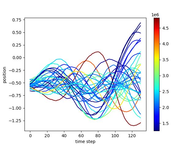
Published in the proceedings of the Workshop on “Structure & Priors in Reinforcement Learning”
at ICLR 2019

tune its internal model of the world and better explain observations. On the other hand the agent will
be driven to visit preferred states which carry little expected free energy.
Formally, an agent entertains a generative model P (õ, ã, s̃) of the environment, which specifies the
joint probability of observations, actions and their hidden causes, where actions are determined by
some policy π. The reader is referred to Appendix A for an overview of the used notation.
If the environment is modelled as a Markov Decision Process (MDP) this generative model factor-
izes as:
                                                T
                                                Y
                  P (õ, ã, s̃) = P (π)P (s0 )   P (ot |st )P (st |st−1 , at )P (at |π)    (1)
                                              t=1

The free energy or Bayesian surprise is then defined as:
                           F = EQ [log Q(s̃) − log P (s̃, õ)]
                              = DKL (Q(s̃)kP (s̃|õ)) − log P (õ)                                  (2)
                              = DKL (Q(s̃)kP (s̃)) − EQ [log P (õ|s̃)]

where Q(s̃) is an approximate posterior distribution. The second equality shows that the free energy
is minimized when the KL divergence term becomes zero, meaning that the approximate posterior
becomes the true posterior, in which case the free energy becomes the negative log evidence. The
third equality then becomes the negative evidence lower bound (ELBO), as we know from variational
autoencoders (VAE) (Kingma & Welling, 2013; Rezende et al., 2014). For a complete derivation the
reader is referred to Appendix B.
In active inference agents pick actions that will result in visiting states of low expected free energy.
Concretely, agents do this by sampling actions from a prior belief about policies according to how
much expected free energy that policy will induce. According to Schwartenbeck et al. (2018) this
means that the probability of picking a policy is given by
                                        P (π) = σ(−γG(π))
                                                    T
                                                    X                                               (3)
                                        G(π) =          G(π, τ )
                                                    τ
where σ is the softmax function with precision parameter γ, which governs the agents goal-
directedness and randomness in its behavior. G is the expected free energy at future time-step τ
under policy π, which can be expanded into:
              G(π, τ ) = EQ(oτ ,sτ |π) [log Q(sτ |π) − log P (oτ , sτ |π)]
                       = EQ(oτ ,sτ |π) [log Q(sτ |π) − log P (oτ |sτ , π) − log P (sτ |π)]         (4)
                        = DKL (Q(sτ |π)kP (sτ )) + EQ(sτ ) [H(P (oτ |sτ ))]
We used Q(oτ , sτ |π) = P (oτ |sτ )Q(sτ |π) and that the prior probability P (sτ |π) is given by a
preferred state distribution P (sτ ). This results into two terms: a KL divergence term between the
predicted states and the prior preferred states, and an entropy term reflecting the expected ambiguity
under predicted states. Action selection in active inference thus entails:
      1. Evaluate G(π) for each policy π
      2. Calculate the belief over policies P (π)
      3. Infer the next action using P (π)P (at+1 |π)
However, examples applying this principle are often limited to cases with a discrete number of
predefined policies, as otherwise calculating P (π) becomes intractable (Friston et al., 2017).

3   N EURAL NETWORKS AS DENSITY ESTIMATORS
In order to overcome the intractability of calculating P (π) we characterize the approximate posterior
with a neural network with parameters φ according to the following factorization:
                                             YT
                                   Q(s̃) =       qφ (st |st−1 , at , ot )
                                            t=1

                                                    2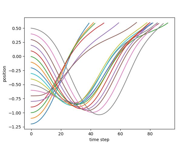
Published in the proceedings of the Workshop on “Structure & Priors in Reinforcement Learning”
at ICLR 2019

Figure 1: The various components of the agent and their corresponding training losses. We minimize
the variational free energy by minimizing both the negative log likelihood of observations and the KL
divergence between the state transition model and the observation model. The inferred hidden state
is characterized as a multivariate Gaussian distribution. Policy learning is achieved by minimizing
the expected free energy G between the state distribution visited by the policy according to the State
Transition Model and the state distribution visited by the expert.

Similarly we parameterise a likelihood model pξ (ot |st ) and dynamics model pθ (st |st−1 , at−1 ) as
neural networks with parameters ξ and θ. These networks output a multivariate Gaussian distribution
with diagonal covariance matrix using the reparametrization trick from Kingma & Welling (2013).
Minimizing the free energy then boils down to minimizing the objective:
         ∀t : minimize : − log pξ (ot |st ) + DKL (qφ (st |st−1 , at , ot )kpθ (st |st−1 , at ))   (5)
                   φ,θ,ξ

The negative log likelihood term of the objective punishes reconstruction error, forcing all informa-
tion from the observations into the state space. The KL term pulls the prior distribution, or the state
transition model, to the posterior model, also known as the observation model, forcing it to learn
to encode state distributions from which observations can be reconstructed without having actual
access to these observations. This can be interpreted as a variational autoencoder (VAE), where
instead of a global prior, the prior is given by the state transition model.
Action selection is then realized by using the state transition model to sample future states, given a
sequence of (randomly sampled) actions. For each action sequence we evaluate G and we execute
the first action of the sequence with minimal G. Any random sampling strategy can be used, for
example the cross entropy method Rubinstein (1996).
The cumbersome sampling according to expected free energy can be avoided by using amortized
inference. In this case we also instantiate a “habit” policy P (at |st ) as a neural network that maps
states to actions in a deterministic or stochastic way. We can train this neural network using back
propagation by minimizing G.
Crucially, we still need to define the preferred states or global prior P (sτ ). When we have access to
a reward signal, this can be converted to a preferred state prior by putting more probability density
on rewarding states. Otherwise, we can initialize the system with a flat prior (each state is equally
preferred), and increase the probability of rewarding states as we visit them. When we have access
to an expert, we can use expert demonstrations to provide a prior on preferred states, i.e. the states
visited by the expert policy. An overview of the various models and train losses is shown in Figure 1.

4    E XPERIMENTS
We validate our theoretical framework on the continuous mountain car problem from the OpenAI
Gym (Brockman et al., 2016), adapted to only provide noisy observations (and no access to the
velocity state). This environment, although quite simple in terms of problem complexity, proves a
good initial trial problem due to greedy approaches failing at it.

                                                     3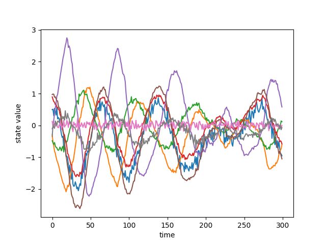
Published in the proceedings of the Workshop on “Structure & Priors in Reinforcement Learning”
at ICLR 2019

      (a) Resulting state space during a role-out.   (b) Predicted observations plotted on top of the ground
                                                     truth observations.

Figure 2: Results of the model training stage. In Figure (a) we see that every parameter of the eight
dimensional state space encodes some element contributing to the prediction. Figure (b) shows
that the models are capable of predicting ground truth observations, indicating that they accurately
learned the environment dynamics.

We instantiate the state transition model, observation model and likelihood models as fully con-
nected neural networks with 64 hidden units. The agent’s internal state is parameterised as an 8
dimensional multivariate Gaussian s. We bootstrap the model by training on a random agent and
optimizing Eq. 5. Our random agent samples actions uniformly in [−1, 1], with a 90% chance of
repeating the previous action. Figure 2a shows a plot of the evolution of the means of the internal
states during a random rollout, whilst Figure 2b shows reconstructions from both the state transition
model and observation model from the same rollout. Note that the state transition model has no
access to any observations. The closeness between ground truth observations and state transition
model reconstructions illustrates that the agent has successfully learned an internal world represen-
tation sufficient to predict the world evolution from a single initial observation.
To construct a preferred state prior, we manually execute 5 “expert rollouts” in the environment.
These rollouts can be seen in Figure 3a. From these rollouts a preferred state distribution is extracted
(Figure 3b). You can see that in the beginning of the sequence, there is a variance on the preferred
states, whereas towards the end the preferred state distribution is peaked around the state reflecting
the car being on the top of the mountain. This is equivalent with a sparse reward signal when
reaching the mountain top at the end of the sequence. Similarly, one can also engineer a preferred
state prior based on the reward signal, which we discuss in Appendix C
We now use this state policy for action selection according the active inference scheme. We sample
random rollouts using the state transition model and calculate the expected free energy G for each.
This indeed selects rollouts that successfully reach the mountain top as shown in Figure 3c. Next,
we also train a policy by minimizing G at every timestep as defined in Eq 4. After training, this
policy is indeed able to generalize to any starting position, consistently reaching the mountain top.

5   R ELATED W ORK

Model-free RL has been successfully proven to work on many game playing (Silver et al., 2016;
Hessel et al., 2017) and robotics problems (Yahya et al., 2017; Kalashnikov et al., 2018). However,
there are still some outstanding challenges, such as the issue of reward engineering (Popov et al.,
2017), generalizing to other environments (Lanctot et al., 2017), and sample inefficiency (Yu, 2018).
Recently there have been promising advancements in the area of model-based RL. Ha & Schmidhu-
ber (2018) train a variational autoencoder (VAE) in conjunction with a recurrent dynamics model to
create a predictive world model. They use this predictive model to train a controller using evolution
strategies (Salimans et al., 2017). Steven Bohez (2018) train jointly a prior and posterior model for
a robotics navigation task. In MERLIN (Wayne et al., 2018), a neural memory module is added on

                                                     4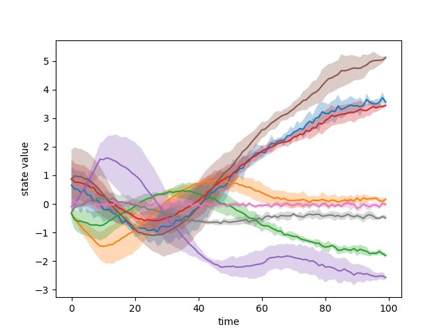
Published in the proceedings of the Workshop on “Structure & Priors in Reinforcement Learning”
at ICLR 2019

    (a) Expert roll-outs from 5 different start posi-        (b) Preferred state distribution from expert roll-
    tions.                                                   outs. Each curve indicates the distribution of a
                                                             latent dimension during rollout.

    (c) Random imaginary rollouts with expected              (d) Actual policy rollouts with different starting
    free energy G, represented in the color bar. Lower       positions.
    G is better.

Figure 3: Results of the policy learning. From expert rollouts (a) we distill a preferred state distri-
bution (b). Sampling imaginary rollouts of the state transition model results in better rollouts having
lower expected free energy G (c). We can use this sampling to train an amortized active inference
policy that successfully solves the environment from any starting position (d).

top of a VAE based dynamics model to facilitate learning policies over longer time windows. In a
similar vein (Srinivas et al., 2018) learns abstract representation for planning.
Instead of using an explicit reward signal, policies can also be learned from demonstrations using
inverse reinforcement learning, basically learning a reward signal from an expert (Ng & Russell,
2000). Another approach for learning from demonstrations is using meta-learning to quickly distill
a policy from a new demonstration (Finn et al., 2017).
Active inference combines elements of all these works into a single theoretical framework. The
preferred states prior can be interpreted as more generic form of value function in RL. It combines
learning world models with action selection and planning. Also, the concept of minimizing expected
Bayesian surprise resembles the work on artificial curiosity for exploration (Graziano et al., 2011).

6    C ONCLUSION

Active inference might underlie the way biological agents perceive and interact with the world.
In this work we show that active inference and the free energy principle can also help artificial
agents interact with the world. Active inference also combines a lot of elements from recent RL
literature, such as building world models, neural planning, artificial curiosity, etc. We belief this is an
interesting direction for further research, to apply this principle to more challenging environments,
such as the ATARI domain or robotics.

                                                         5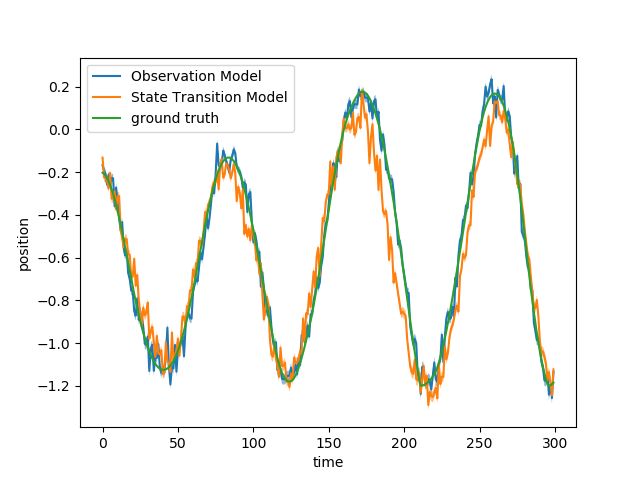
Published in the proceedings of the Workshop on “Structure & Priors in Reinforcement Learning”
at ICLR 2019

ACKNOWLEDGMENTS
Ozan Catal is funded by a Ph.D. grant of the Flanders Research Foundation (FWO).

R EFERENCES
Greg Brockman, Vicki Cheung, Ludwig Pettersson, Jonas Schneider, John Schulman, Jie Tang, and
  Wojciech Zaremba. Openai gym. CoRR, abs/1606.01540, 2016. URL http://arxiv.org/
  abs/1606.01540.

Chelsea Finn, Tianhe Yu, Tianhao Zhang, Pieter Abbeel, and Sergey Levine. One-shot visual imi-
  tation learning via meta-learning. CoRR, abs/1709.04905, 2017. URL http://arxiv.org/
  abs/1709.04905.

Karl Friston. The free-energy principle: A unified brain theory? Nature Reviews Neuroscience, 11
  (2):127–138, 2010. ISSN 1471003X. doi: 10.1038/nrn2787. URL http://dx.doi.org/
  10.1038/nrn2787.

Karl Friston, James Kilner, and Lee Harrison. A free energy principle for the brain. Journal of
  Physiology Paris, 100(1-3):70–87, 2006. ISSN 09284257. doi: 10.1016/j.jphysparis.2006.10.001.

Karl Friston, Spyridon Samothrakis, and Read Montague. Active inference and agency: Optimal
  control without cost functions. Biological Cybernetics, 106(8-9):523–541, 2012. ISSN 03401200.
  doi: 10.1007/s00422-012-0512-8.

Karl Friston, Philipp Schwartenbeck, Thomas FitzGerald, Michael Moutoussis, Timothy Behrens,
  and Raymond J. Dolan. The anatomy of choice: active inference and agency. Fron-
  tiers in Human Neuroscience, 7(September):1–18, 2013. ISSN 1662-5161. doi: 10.3389/
  fnhum.2013.00598. URL http://journal.frontiersin.org/article/10.3389/
  fnhum.2013.00598/abstract.

Karl Friston, Thomas FitzGerald, Francesco Rigoli, Philipp Schwartenbeck, and Giovanni Pezzulo.
  Active inference: A Process Theory. Neural Computation, 29:1–49, 2017. ISSN 1530888X. doi:
  10.1162/NECO a 00912.

Vincent Graziano, Tobias Glasmachers, Tom Schaul, Leo Pape, Giuseppe Cuccu, Juxi Leitner, and
  Jrgen Schmidhuber. Artificial curiosity for autonomous space exploration. Acta Futura, pp. 41–
  51, 01 2011.

David Ha and Jürgen Schmidhuber. World Models. arXiv preprint, 2018. doi: 10.5281/zenodo.
  1207631. URL http://arxiv.org/abs/1803.10122{%}0Ahttp://dx.doi.org/
  10.5281/zenodo.1207631.

Matteo Hessel, Joseph Modayil, Hado van Hasselt, Tom Schaul, Georg Ostrovski, Will Dabney, Dan
 Horgan, Bilal Piot, Mohammad Azar, and David Silver. Rainbow: Combining Improvements
 in Deep Reinforcement Learning. arXiv preprint, 2017. URL http://arxiv.org/abs/
 1710.02298.

Dmitry Kalashnikov, Alex Irpan, Peter Pastor, Julian Ibarz, Alexander Herzog, Eric Jang, Deirdre
 Quillen, Ethan Holly, Mrinal Kalakrishnan, Vincent Vanhoucke, and Sergey Levine. Qt-opt: Scal-
 able deep reinforcement learning for vision-based robotic manipulation. CoRR, abs/1806.10293,
 2018. URL http://arxiv.org/abs/1806.10293.

Diederik P. Kingma and Max Welling. Auto-encoding variational bayes. CoRR, abs/1312.6114,
  2013. URL http://arxiv.org/abs/1312.6114.

Marc Lanctot, Vinı́cius Flores Zambaldi, Audrunas Gruslys, Angeliki Lazaridou, Karl Tuyls, Julien
 Pérolat, David Silver, and Thore Graepel. A unified game-theoretic approach to multiagent rein-
 forcement learning. CoRR, abs/1711.00832, 2017. URL http://arxiv.org/abs/1711.
 00832.

                                               6
Published in the proceedings of the Workshop on “Structure & Priors in Reinforcement Learning”
at ICLR 2019
Andrew Y. Ng and Stuart J. Russell. Algorithms for inverse reinforcement learning. In Proceedings
of the Seventeenth International Conference on Machine Learning, ICML ’00, pp. 663–670, San
Francisco, CA, USA, 2000. Morgan Kaufmann Publishers Inc. ISBN 1-55860-707-2. URL
http://dl.acm.org/citation.cfm?id=645529.657801.
Ivaylo Popov, Nicolas Heess, Timothy P. Lillicrap, Roland Hafner, Gabriel Barth-Maron, Matej
Vecerik, Thomas Lampe, Yuval Tassa, Tom Erez, and Martin A. Riedmiller. Data-efficient deep
reinforcement learning for dexterous manipulation. CoRR, abs/1704.03073, 2017. URL http:
//arxiv.org/abs/1704.03073.
Danilo Jimenez Rezende, Shakir Mohamed, and Daan Wierstra. Stochastic backpropagation and
approximate inference in deep generative models. In Eric P. Xing and Tony Jebara (eds.), Pro-
ceedings of the 31st International Conference on Machine Learning, volume 32 of Proceedings
of Machine Learning Research, pp. 1278–1286, Bejing, China, 22–24 Jun 2014. PMLR. URL
http://proceedings.mlr.press/v32/rezende14.html.
Reuven Y. Rubinstein. Optimization of computer simulation models with rare events. European
Journal of Operations Research, 99:89–112, 1996.
Tim Salimans, Jonathan Ho, Xi Chen, Szymon Sidor, and Ilya Sutskever. Evolution Strategies as
a Scalable Alternative to Reinforcement Learning. arXiv preprint, pp. 1–13, 2017. ISSN 1744-
4292. doi: 10.1.1.51.6328. URL http://arxiv.org/abs/1703.03864.
Philipp Schwartenbeck, Johannes Passecker, Tobias Hauser, Thomas H B FitzGerald, Martin Kro-
nbichler, and Karl J Friston. Computational mechanisms of curiosity and goal-directed explo-
ration. bioRxiv, pp. 411272, 2018. doi: 10.1101/411272. URL https://www.biorxiv.
org/content/early/2018/09/07/411272.
David Silver, Aja Huang, Chris J. Maddison, Arthur Guez, Laurent Sifre, George Van Den Driess-
che, Julian Schrittwieser, Ioannis Antonoglou, Veda Panneershelvam, Marc Lanctot, Sander
Dieleman, Dominik Grewe, John Nham, Nal Kalchbrenner, Ilya Sutskever, Timothy Lillicrap,
Madeleine Leach, Koray Kavukcuoglu, Thore Graepel, and Demis Hassabis. Mastering the game
of Go with deep neural networks and tree search. Nature, 529(7587):484–489, 2016. ISSN
14764687. doi: 10.1038/nature16961.
Aravind Srinivas, Allan Jabri, Pieter Abbeel, Sergey Levine, and Chelsea Finn. Universal Planning
Networks. Proceedings of the 35th International Conference on Machine Learning, Stockholm,
Sweden, PMLR, 2018. ISSN 1938-7228. URL http://arxiv.org/abs/1804.00645.
Sam Leroux Elias De Coninck Bert Vankeirsbilck Pieter Simoens Bart Dhoedt Steven Bohez,
Tim Verbelen. Robot navigation using a variational dynamics model for state estimation and
robust control. In Deep RL workshop NeurIPS 2018, December 2018.
Greg Wayne, Chia-Chun Hung, David Amos, Mehdi Mirza, Arun Ahuja, Agnieszka Grabska-
Barwinska, Jack Rae, Piotr Mirowski, Joel Z. Leibo, Adam Santoro, Mevlana Gemici, Malcolm
Reynolds, Tim Harley, Josh Abramson, Shakir Mohamed, Danilo Rezende, David Saxton, Adam
Cain, Chloe Hillier, David Silver, Koray Kavukcuoglu, Matt Botvinick, Demis Hassabis, and
Timothy Lillicrap. Unsupervised Predictive Memory in a Goal-Directed Agent. arXiv preprint,
2018. URL http://arxiv.org/abs/1803.10760.
Ali Yahya, Adrian Li, Mrinal Kalakrishnan, Yevgen Chebotar, and Sergey Levine. Collective robot
reinforcement learning with distributed asynchronous guided policy search. In IEEE Interna-
tional Conference on Intelligent Robots and Systems, volume 2017-Septe, pp. 79–86, 2017. ISBN
9781538626825. doi: 10.1109/IROS.2017.8202141.
Yang Yu. Towards sample efficient reinforcement learning. In Proceedings of the Twenty-Seventh
International Joint Conference on Artificial Intelligence, IJCAI-18, pp. 5739–5743. International
Joint Conferences on Artificial Intelligence Organization, 7 2018. doi: 10.24963/ijcai.2018/820.
URL https://doi.org/10.24963/ijcai.2018/820.
7Published in the proceedings of the Workshop on “Structure & Priors in Reinforcement Learning”
at ICLR 2019
Appendices
A G LOSSARY
Definition Description
st State at time t
ot Observation at time t
at Action at time t
sτ Expected state at a future timestep τ
s̃ Sequence of states
õ Sequence of observations
ã Sequence of actions
P (õ, ã, s̃) Generative model of the agent
P (ot |st ) Likelihood model
π Policy
P (st |st−1 , at−1 ) State transition model
P (at |π) Action at time t given a policy
P (π) Belief over policies
P (s̃|õ) True posterior about hidden states given a se-
quence of observations
Q(s̃) Approximate posterior about hidden states
F = EQ(s) [log Q(s̃) − log P (s̃, õ)] Free energy
G(·) P Expected free energy
σ(z)j = ezj / k ezk Softmax or Boltzmann distribution
γ Precision parameter governing goal-directedness
and randomness
Table 1: Glossary table with brief description of the used terms and their definitions
8Published in the proceedings of the Workshop on “Structure & Priors in Reinforcement Learning”
at ICLR 2019
B F REE ENERGY DERIVATION
Starting from the definition of free energy:
s) − log P (e
F = EQ [log Q(e s, o
e)]
where Q(e
x) is an approximate posterior distribution. We can expand the free energy F as follows:
s) − log P (e
F = EQ [log Q(e s, o
e)]
s) − log P (e
= EQ [log Q(e s|e
o) − log P (e
o)]
= DKL (Q(e x|e
s)kP (e o)) − log P (e
o),
Similarly, we can also rewrite the free energy expression as:
F = EQ [log Q(es) − log P (e
s, o
e)]
using the identity P (e
s, o o|e
e) = P (e s)P (e
s)
= EQ [log Q(es) − log P (e
s) − log P (e
o|e
s)]
= DKL (Q(e s)kP (es)) − EQ [log P (e
o|e
s)]
C A REWARD - BASED PREFERRED STATE PRIOR
In a traditional RL setting, an agent only has access to a reward signal, rather than expert demon-
strations. In this case the agent will need to find the preferred state prior that matches the reward
signal (higher probability for states that yield higher reward), which is equivalent to learning a value
function V (·) in RL. In the mountain car problem, only a sparse reward of +1 is given when reaching
the top of the mountain. Based on this reward function, we can define the preferred state distribution
as a Gaussian centered around the states where the car reaches the top of the mountain after timestep
100. We can use this prior instead of the one induced by the demonstrations for active inference. We
see in Figure 4 that again trajectories reaching the top result in the lowest expected free energy.
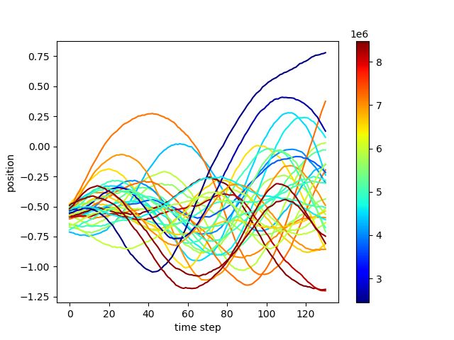
Figure 4: Random imaginary rollouts with corresponding expected free energy G when the preferred
state is defined as those states that give reward. Lower G is better.
9You can also read