Polarization dynamics of ultrafast solitons - arXiv.org

Polarization dynamics of ultrafast solitons
 AVI K LEIN , 1 S ARA M EIR , 1 H AMOOTAL D UADI , 1 A RJUNAN
 G OVINDARAJAN , 2 AND M OTI F RIDMAN 1,*
 1 Faculty of Engineering and the Institute of Nanotechnology and Advanced Materials, Bar-Ilan
 University, Ramat Gan 5290002, Israel
arXiv:2104.08937v1 [physics.optics] 18 Apr 2021

 2 Centre for Nonlinear Dynamics, School of Physics, Bharathidasan University, Tiruchirappalli 620 024,
 India
 * mordechai.fridman@biu.ac.il

 Abstract: We study the polarization dynamics of ultrafast solitons in mode-locked fiber
 lasers. We find that when a stable soliton is generated, it’s state-of-polarization shifts toward a
 stable state and when the soliton is generated with excess power levels it experiences relaxation
 oscillations in its intensity and timing. On the other hand, when a soliton is generated in an
 unstable state-of-polarization, it either decays in intensity until it disappears, or its temporal
 width decreases until it explodes into several solitons and then it disappears. We also found that
 when two solitons are simultaneously generated close to each other, they attract each other until
 they collide and merge into a single soliton. Although, these two solitons are generated with
 different states-of-polarization, they shift their state-of-polarization closer to each other until the
 polarization coincides when they collide. We support our findings by numerical calculations of a
 non-Lagrangian approach by simulating the Ginzburg-Landau equation governing the dynamics
 of solitons in a laser cavity. Our model also predicts the relaxation oscillations of stable solitons
 and the two types of unstable solitons observed in the experimental measurements.

 © 2021 Optical Society of America under the terms of the OSA Open Access Publishing Agreement

 1. Introduction
 Ultrafast fiber lasers have revolutionized the industry with their high efficiency, robustness, tune-
 ability, and easy in assembling [1]. These lasers are implemented in high speed communication
 systems, quantum communication schemes, and for precision material processing [2]. The
 mode-locking process in these fiber lasers is done either by introducing a saturable absorber into
 the cavity or by relying on the Kerr effect in the fiber. One of the simplest and most reliable
 methods for mode-locking is based on the polarization mode dispersion in the fiber [3–12].
 In mode-locking schemes which are based on the polarization mode dispersion, polarization
 controllers in the cavity induce birefringence, followed by a polarizer [3, 4]. When a pulse with
 high power levels is traveling in the fiber, it changes the birefringence of the fiber via the Kerr
 effect leading to a higher transmission through the polarizer [13–17]. While this method requires
 to adjust the polarization controller once in a while, it is highly robust and gives a consistent
 output pulse shape and spectrum [3,4]. Therefore, this method for mode-locking is implemented
 in many fiber lasers [18]. It is more stable, there is no degradation of the saturable absorber
 material over time, it is fully embedded in the fiber, it is based on off-the-shelf components, and
 it is suitable for wide bandwidth of frequencies [2, 19].
 However, while the polarization dynamics of the pulse play an important role in these types of
 ultrafast fiber lasers, the evolution inside the cavity is not fully understood yet. In order to identify
 the appropriate dynamics, different models were developed for such lasers. These include the
 numerical evolution of the scalar Ginzburg-Landau equations [20–23] or analytical solutions for
 these equations [24]. Some numerical works have focused on the state-of-polarization dynamics
 of the output of ultrafast lasers [25–34] and others described the state-of-polarization during the
 propagation of the pulse inside the laser cavity [35–37]. The polarization dynamics of pulses

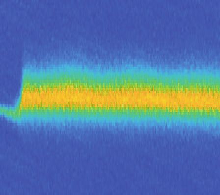
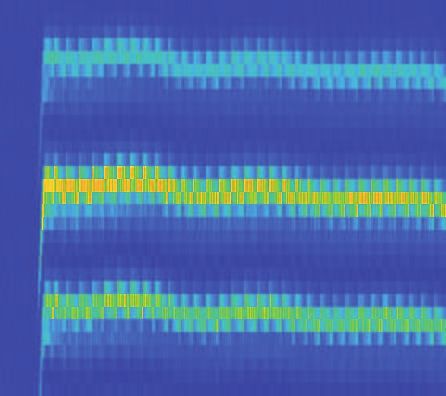
in the laser are also responsible for ultrafast phenomena after the solitons are generated [38, 39],
including, soliton oscillations [40–44], solitons expulsions [45], soliton accelerations, unstable
solitons [46–48], and the formation of soliton molecules [49–53].
 Nevertheless, measuring the soliton dynamics is a challenging task due to the limited temporal
resolution of electronic detectors. Thus, the slow electronic measurements of vector solitons
in fiber lasers were combined with optical spectrometer measurements [54–59] or with RF
spectrometer measurements [60, 61]. Faster spectral measurements, which do not average over
many round-trips, were demonstrated with a time-stretch system [62–68]. By combining the
time-stretch system with a time-lens, it is possible to obtain a high temporal resolution together
with a high spectral resolution after every round-trip [69]. However, none of these methods
measured the state-of-polarization with high temporal resolution. Also, the time-lens and time-
stretch methods can not measure the dynamics of the laser before the soliton is formed.
 To unwrap these hindrances, we have developed a full-Stokes temporal imaging system with
a 0.5 temporal resolution and a 30 field of view dedicated for studying the polarization
dynamics of solitons in fiber lasers. Our system retrieves the intensity, phase, and state of
polarization of the signal with a high temporal resolution by combining the measurements from
slow detectors, three time-lenses and a time-stretch. The system is also equipped with an optical
buffer for measuring the polarization dynamics of the noise before the pulse is formed. This
is important for investigating the process of mode-locking polarization dynamics in such fiber
lasers.

2. Experimental setup and the mode-locking dynamics in fiber laser
Our system, shown in Fig. 1(a), measures the signal in three different channels. The first channel
has a low resolution measurement with a photo-detector, which allows to detect temporal shifts
beyond 100 round trips with a temporal resolution of 50 . The second channel has a time-
stretch system for spectral detection of the signal in real-time with a spectral resolution of
0.2 [70, 71]. The third channel has an array of three time-lenses, measuring the state of
polarization evolution with a 0.5 resolution [72, 73]. The time-lens channel is also equipped
with an optical buffer for storing the incoming signal in a long fiber. This enable us to analyze
the signal once the laser gets stabilized, therefore, it is suitable for measuring the dynamics
of signals with unknown time-of-arrival, such as, the mode-locking process of the laser. By
combining the measurements from the time-stretch together with the time-lenses, we can retrieve
the phase of the input signal with a high temporal resolution as illustrated in Fig. 1(a) [69, 74].
 With this system, we measure and analyze the polarization dynamics during the polariza-
tion mode-locking process of the laser. We generate solitons with excess power levels and
observe their relaxation oscillations. We also detect unstable solitons when the soliton state of
polarization is far from the mode-locking state of polarization, and analyze their two different
types. These include one type of unstable solitons which decay and disappear and other type of
unstable solitons which explode and then disappear. We also measure the collision dynamics of
two solitons merging into one and detect how the state-of-polarization of each soliton is shifting
toward the other.
 We start with investigating the polarization mode-locking process of fiber lasers. While in
the spectral domain, there are ultrafast measurements of the mode-locking process [62–67], it is
challenging to measure it in the time-domain and only scalar measurements were done without
measuring the ultrafast polarization dynamics [69]. However, since the mode-locking process
is based on polarization rotation inside the cavity [1], it is essential to measure the ultrafast
polarization dynamics in the time domain. We measure the spectral, temporal, and polarization
ultrafast dynamics of the mode-locking process with our system. The results as a function of the
round-trip number are shown in Fig. 1, where Fig. 1(b) shows the low resolution measurement,
Fig. 1(c) shows the spectral measurement by the time-stretch, and Fig. 1(d) shows the output

-2 0.2 6
(a) Laser pump (b) (e)
 PC EDF

 Time [ns]

 Bandwidth [nm]
 WDM

 Intensity [a.u]
 0

 0.1 3
 Laser Scope
 Poloraizer Isolator 2
 1540
 PC (c)

 Wavelength [nm]
 90% OC 0 0
 10% 1550 -1000 -500 0 500 1000
 Low resolution SMFi Round trips
 S3
 20 km SMF (f)
 Time stretch BPF 1560 0.4 S2

 -4 (d)
 DCFp pump preparation
 Round trip 0
 HNLF
 Pump

 Time [ns]
 0.3
 WDM WDM -2

 S3
 Time lens Signal DCFs 0 Round trip -100
 0.2

 Optical buffer 2
 pulse splitter -1000 0 1000 0.3 0.4 0.5
 Round trips S2

 Fig. 1. (a) Experimental setup for measuring the temporal, spectral, and polarization
 dynamics of solitons in polarization mode-locked fiber laser. Ultrafast fiber laser with
 a polarizer as a saturable absorber. The output from the laser splits into three arms,
 a direct measurement with low resolution, a time-stretch scheme for measuring the
 spectrum, and full-Stokes time-lenses for measuring the intensity with high temporal
 resolution as well as the polarization dynamics. (b) - (d) Measurements of the mode-
 locking process in the fiber laser. (b) Direct low resolution measurement showing
 that the intensity of the peak increases when the laser mode-locked. (c) Spectral
 measurement showing the broadening in the spectrum and Kelly sidebands during the
 mode-locking process, indicating the formation of solitons in the laser. (d) The output
 from the three time-lenses indicating the polarization dynamics during the mode-
 locking process. (e) Pulse intensity (blue curve) and spectral bandwidth (red curve) of
 the laser output as a function of round-trips in the cavity. (f) State of polarization of
 the pulse during the 100 round trips before the mode-locking.

from the three time-lenses. We denote the timing of mode-locking as round-trip number 0. All
these measurements are acquired by a fast oscilloscope with deep memory where the data set is
segmented equally to the different round-trips. Therefore, when the segments duration equal to
the repetition-rate, we observe a horizontal line since the pulse arrives at the same time at each
segment, which is evident in Fig. 1(b) after mode-locking. Before the mode-locking, the pulse
timing is shorter and therefore we observe a linear shift. The linear shift before the mode-locking
indicates that the round-trip time is shorter by 0.62 than after mode-locking. This change in
the round-trip time results from the Kerr-effect generated by the high peak power of the mode-
locked laser of 30 over the 13.3 long cavity. Based on these results, we evaluate the change
 ¤ −20 2 / which coincides with the known
in the index of refraction of the glass to be Δ = 310
Kerr value of fused silica [75]. The spectrum of the pulse, shown in Fig. 1(c), has a width of
6 after the mode locking with Kelly sidebands, which agrees with a 0.5 soliton width. We
have also evaluated the intensity and bandwidth of the pulse after every round-trip and shown
these results in Fig. 1(e). From the three time-lenses measurements, shown in Fig. 1(d), we
obtained the state of polarization dynamics during the mode-locking process [72]. The state of
polarization of the soliton during the mode-locking process is shown in Fig. 1(f) on a Poincare
sphere representation. From these results, we identify a specific stable state-of-polarization
which the laser tends to prefer, serves as an attractor for the state-of-polarization.

3. Soliton polarization dynamics
Next we investigate solitons with higher power levels. When the soliton is formed with an excess
power level, we observe temporal and intensity relaxation oscillations of the single soliton.

Soliton oscillations were shown in multi soliton structures known as soliton molecules where
the tail of one soliton serves as an effective potential for its adjacent soliton [49–53]. Single
solitons are also expected to oscillate but their oscillations are bellow the temporal resolution
of current detectors. While the oscillations of two solitons are easily detected by fringes in
the spectrum [40–44], the oscillations of a single soliton are below the temporal resolution of
current detectors. We utilize our system to measure the temporal oscillations of a single soliton.
These oscillations are generated when a soliton starts with excessive power levels and so its
power oscillates [40–44], similar to the relaxation oscillations in the output power of lasers
when starting to lase. Due to these oscillations in the power level of the soliton, the soliton
timing oscillates as well due to the Kerr effect. We have generated such solitons and measured
their oscillations in time and intensity. Although, the low resolution and spectral measurements
shown in Figs. 2(a) and (b) do not reveal any temporal oscillations, the high-resolution time-
lens measurements presented in Fig. 2(c) are showing the temporal oscillations. The time-lens
measurements during the formation of the solitons are shown in Fig. 2(d) and by comparing
the intensity from the three time-lenses, we obtain the shift in the state-of-polarization during
the formation of the solitons. From this ramification, we predict that during the formation of
the soliton the state-of-polarization is shifting but during the relaxation oscillations, the state-
of-polarization is stable. By integrating the power in the spectral measurements, we also obtain
the intensity of the soliton as a function of round-trip and find that it too oscillates and the
oscillation amplitude decays similar to the relaxation oscillations of lasers. To emphasize the
oscillation dynamics, we plot the temporal and intensity oscillations in Fig. 2(f), where we
evaluate the power and timing of the soliton as a function of the round-trip number. The shift
of 30% in the pulse intensity during the oscillations agrees with a shift of 40 in the soliton
timing over 2000 round-trips due to the Kerr effect. The soliton timing, denoted by the red curve,
indicates the change in the soliton timing compared to the segment duration, therefore, the pulse
time-of-arrival is the derivative of the red curve, leading to the /4 shift between the blue and
the red curves. We have also developed a semi-analytical model predicting these oscillations
which is presented in the appendix.
 -2 (e) 1 6
 (a) -1 (d)
 (c)
 (f)
 Time [ns]

 -1 S3
 Time [ns]

 0 S1
 Soliton timing [ps]
 0
 1 RT 0 0.9
 Intensity [a.u]

 1
 2 0
 2 RT -100
 Wavelength [nm]

 1540 (b) -100 0 0.8
 -1 (c)
 Time [ns]

 1550
 0
 0.7 -6
 1
 1560 0 10000 20000
 0 10000 0 10000
 Round trips Round trips Round trips

 Fig. 2. Measured soliton dynamics showing temporal oscillations with decreasing
 amplitude both in time and intensity as a function of the round-trip number. (a)
 Low resolution measurement of the generated soliton. (b) Spectral measurement
 showing the broadening in the spectrum when the soliton is generated. (c) Time-lens
 measurement of the soliton showing the temporal oscillations in the soliton timing.
 The constant ratio between the three time-lenses indicate that the state-of-polarization
 is constant during the oscillations. (d) A zoom-in measurement of the time-lens results
 during the soliton formation. (e) The state-of-polarization of the soliton during its
 formation, showing a shift until reaching a stable state-of-polarization where it stays
 during the oscillations. RT - round trip. (f) The soliton peak intensity and timing as a
 function of the round-trip number.

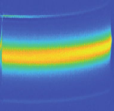
Next, we study unstable solitons which are generated in different states-of-polarization than
the stable ones. Such unstable solitons were predicted by numerical calculations [46–48], and
were measured with slow detectors [68] or in the spectral domain [45, 69]. Nevertheless, with
our system, we measured not only the spectral and temporal characteristics but also the ultrafast
polarization dynamics of such unstable solitons and classify their two different types. The first
type of unstable solitons decays in its intensity until disappearing and the second type shrinks in
its temporal width until it explodes into several solitons which then disappear. We present the
time-lens measurements of these solitons in Figs. 3(a) and (c) and their spectral measurements
in Figs. 3(b) and (d). In the first type, we observe an accelerating soliton as seen by the curve
trajectory shown in Fig. 3(a). The intensity of the soliton is constant as evident by the spectral
measurement shown in Fig. 3(b), and then disappears in 50 round trips. In the second type we
observe the same accelerating soliton, as shown in Figs. 3(c) and (d). But, at the last 50 round
trips the soliton explodes into several solitons as evident by the zoom-in measurements shown in
Figs. 3(e) and (f). The explosion is evident both from the temporal and spectral measurements.
We also analyze the state-of-polarization of the unstable solitons and observe that as the solitons
resonate in the cavity, their states-of-polarization drift until the solitons disappear, as seen in
Fig. 3(g). It is worthwhile to mention that our semi-analytical model, which is presented in the
appendix, predicts these two types of unstable solitons.

 Type 1 Type 2
 -3 (a) (c) (e) (g)
 S3
 Wavelength [nm] Time [ns]

 -2
 Type 2
 -1
 0
 1 S1

 1549 (b) (d) (f)

 1550
 Type 1
 1551

 0 5000 0 10000 10800 10850
 Round trips Round trips Round trips

 Fig. 3. Unstable solitons showing accelerated solitons with drifting states-of-
 polarization that suddenly disappear. We observe two types of unstable solitons, first
 type which accelerate and disappear and the second type which accelerate, explodes
 into several solitons and then disappear. (a) and (b) the intensity and spectrum of the
 first type of the unstable soliton as a function of the round-trip number. (c) and (d)
 the intensity and spectrum of the second type of the unstable soliton as a function of
 the round trip number. (e) and (f) zoom-in of insets (c) and (d), respectively, showing
 the temporal and spectral dynamics of the exploding soliton and its disappearance. (g)
 The state-of-polarization of both unstable solitons on a Poincare sphere representation.

 Finally, we study the collision dynamics of two solitons that are merging into a single one. In
the existing studies, solitons collisions were measured in the spectral domain [50–52, 63–65] or
with a time-lens but without the polarization dynamics [69]. However, numerical simulations
predict reach dynamics in the picosecond time-scales [49, 51]. Here we utilize our time-lenses
to measure the polarization dynamics of two solitons generated with 2 ps temporal separation
which then merge into a single soliton. The measured results are shown in temporal and spectral
scales in Fig. 4(a) and (b). The two solitons start at a temporal separation of 2 and move
closer to each other at each round-trip until they collide around round-trip number 1000. These
findings are supported by the spectral fringes indicating a soliton collision as shown in Fig. 4(b),
where the spectral fringes are getting wider until they disappear at round-trip number 1000.

(a) (b) 1545

 Wavelength [nm]
 1000
 1550

 s
 trip
 500

 nd
 Rou
 -3 -2 -1 0 1555
 0 1 2 3 0 1000
 Time [ps] Round trips

 Fig. 4. Two solitons colliding into a single soliton. (a) High resolution temporal image
 of the solitons showing two solitons with a 2 temporal separation merging into a
 single soliton after 1000 round-trips. (b) The spectrum of colliding solitons measured
 by the time-stretch system showing fringes where their periodicity reduces as expected
 in the case of a collision scenario of two temporarily separated solitons.

 To understand the polarization dynamics during the collision, we analyze the temporal
measurements of the three time-lenses which are presented in Fig. 5(a) in order to obtain the
state-of-polarization of each soliton after each round-trip. The two solitons start with different
states-of-polarization and as they move closer, their states-of-polarization shift one toward the
other until the solitons merge. This dynamics of the state-of-polarization of the soliton is shown
in Fig. 5(b), where the state-of-polarization of one soliton is indicated by the blue dots and the
state-of-polarization of the other soliton is indicated by the red dots. The state-of-polarization
of the merged soliton is denoted by the purple dots.

 (a) (b) S3

 -1 S1
 RT 700
 Time [ns]

 0.1

 0
 RT 1000
 -0.1 0 0.2 0.3 0.4
 1
 -0.1
 RT 100 RT 1140
 S3
 Stoke vector of the right pulse
 0 1000 S1 Stoke vector of the left
 Round trips Stoke vector of the combined

 Fig. 5. (a) The temporal measurements of the three time-lenses showing the collision
 of two solitons merging into a single soliton. The results of the first time-lens are at
 around −1 , the results of the second are at around 0 and the results of the third
 are at around 1 (b) The state-of-polarization of both solitons before and after the
 collision into a single soliton. The state-of-polarization of the right soliton is denoted
 by the blue dots and the state-of-polarization of the left soliton is denoted by the red
 dots. The combined soliton after the collision is denoted by the purple dots. RT -
 round trip.

4. Conclusions
To conclude, we investigated the polarization dynamics of solitons in mode-locked fiber laser
with high temporal and spectral resolutions. We studied the polarization dynamics during the
formation of solitons, and observed relaxation oscillations in the intensity and timing of the
solitons after formation. We found the state-of-polarization of stable and unstable solitons,
detected their polarization dynamics, and identified two types of unstable solitons. Finally, we
observed the polarization dynamics of two solitons while they collided and merged into a single

soliton. These experimental findings are supported by a semi-analytical approach known as
non-Lagrangian method which agrees well with the experimental measurements. We believe
that our findings can provide a deep insight into the generation and control of nonlinear localized
structures and their collision dynamics which can pave a new avenue in maneuvering solitons in
fiber lasers for multifaceted lightwave applications.

Appendix
In order to model our system, we resort to a non-Lagrangian approach for simulating coupled
complex Ginzburg-Landau equations for the two components of the electric wave vector as for
the first state-of-polarization [20]:

 2 2 4 3 
 + + | | = + | | + + , (1)
 2 3
and for the second state-of-polarization:

 2 2 4 3 
 + + | | = + | | + + . (2)
 2 3
It is to be noted that the terms and are complex. Here, the real part of denotes the wave
dispersion, the imaginary part of is to note the spectral filtering coefficient. Similarly, the real
part of refers to the third order dispersion, and the imaginary part of indicates the cubic
frequency dependent of the gain or loss coefficient. Also, the nonlinear coefficient is represented
through the term , and denotes the high order correction terms. The other system parameters
such as refers to the linear gain and frequency shifts, and the coupling between the two modes
is denoted by . In this model, we neglect the nonlinear coupling terms between the different
states-of-polarization during the propagation in the nonlinear fiber laser. Instead, we include the
linear coupling term which can arise from the polarization controllers in the cavity. We also
assume that the linear coupling strength is stronger than the nonlinear coupling strength. In this
model, we assume two solitons in the two states-of-polarization which are described by these
functions as given below:
 ( − 2 ) 2
 − 4
 2 ( − 2 ) 2 + 5 ( − 2 )+ 6
 1 = 1 3 2
 (3)
 ( − 2 ) 2
 − 4
 2 ( − 2 ) 2 + 5 ( − 2 )+ 6
 2 = 1 3 2

where 1 and 1 denote the amplitude, 2 and 2 indicate the timing, 3 and 3 refer to the
temporal width, 4 and 4 is for the frequency chirp, 5 and 5 represents the frequency, and 6
and 6 are the phases for the two components. The model reveals the change in each components
as a function of round-trips in the cavity and therefore we can observe amplitude and temporal
shifts. By considering the relative phase between the two states of polarization and the amplitude
of each state of polarization, we obtain the state of polarization of the output pulse. This model
reveals all the ultrafast phenomena we observed in the experiment including the relaxation
oscillations, unstable solitons, and solitons collisions. However, this model is not suitable for
analyzing the dynamics before the soliton gets generated or after it disappears or explodes as
expected.
 We start by simulating a soliton in a stable state-of-polarization and observe relaxation
oscillations in the intensity and in the timing of the soliton. These results are delineated in
Fig. 6(a) and agree well with the measured results presented in Fig. 2. Next, we find the states
of polarization for unstable solitons of the two types discussed earlier. The dynamics of the
first type is shown in Fig. 6(b). We can observe a reduction in the intensity while the soliton

accelerates. Similarly, the dynamics of the unstable soliton from the second type is shown in
Fig. 6(c). Here the soliton intensity gets increased while its width decreases leading to a soliton
explosion. As our model assumes one soliton in each state-of-polarization, the soliton explosion
into more solitons is out of the scope of our model. Note that these results are similar to the
measured results obtained in our laser. However we would like to mention that a small difference
in the starting state-of-polarization of the soliton determines whether the unstable soliton is of
the first type or of the second type. All the MATLAB codes for generating these results are
available online.
 2 1 1 6 3
 (a) (b) (c)
 10

 Temporal width [ps]
 Intensity [a.u]

 Intensity [a.u]
 Intensity [a.u]

 Timing [ps]

 Timing [ps]
 0 3

 1 -10
 0 0 0 0
 500 1000 0 100 0 300
 Round trips Round trips Round trips

 Fig. 6. Calculated results of single solitons in fiber laser cavity represented by
 the Ginzburg-Landau equation. (a) Stable soliton generated in the stable state-of-
 polarization exhibiting relaxation oscillations in the intensity and in timing which
 agrees with the experimental measurements. (b) Unstable soliton of the first type gen-
 erated in an unstable state-of-polarization showing intensity decay while accelerating
 in time indicated by the red curve which agrees with the experimental measurements.
 (c) Unstable soliton of the second type showing a rapid increase in the intensity together
 with decrease in the soliton temporal width indicating a soliton explosion.

Disclosures
The authors declare no conflicts of interest.

References
1. E. P. Ippen, “Principles of passive mode locking,” Appl. Phys. B 58, 159–170 (1994).
2. M. E. Fermann and I. Hartl, “Ultrafast fiber laser technology,” IEEE J. Sel. Top. Quantum Electron. 15, 191–206
 (2009).
3. M. Fermann, M. Andrejco, Y. Silberberg, and M. Stock, “Passive mode locking by using nonlinear polarization
 evolution in a polarization-maintaining erbium-doped fiber,” Opt. letters 18, 894–896 (1993).
4. L. E. Nelson, D. Jones, K. Tamura, H. Haus, and E. Ippen, “Ultrashort-pulse fiber ring lasers.” Appl. Phys. B: Lasers
 & Opt. 65 (1997).
5. R. Gumenyuk and O. G. Okhotnikov, “Temporal control of vector soliton bunching by slow/fast saturable absorption,”
 JOSA B 29, 1–7 (2012).
6. A. Kim, D. Yong, K. Spaulding, and J. Kutz, “Control of pulse-train uniformity with passive polarizers in mode-
 locked optical fiber lasers,” in Nonlinear Optics: Materials, Fundamentals and Applications, (Optical Society of
 America, 2000), p. ThB25.
7. L. Zhao, C. Lu, H. Y. Tam, P. K. A. Wai, and D. Tang, “High fundamental repetition rate fiber lasers operated in
 strong normal dispersion regime,” IEEE Photonics Technol. Lett. 21, 724–726 (2009).
8. C. Mou, H. Wang, B. G. Bale, K. Zhou, L. Zhang, and I. Bennion, “All-fiber passively mode-locked femtosecond
 laser using a 45º-tilted fiber grating polarization element,” Opt. express 18, 18906–18911 (2010).
9. X. Liu, F. Ilday, K. Beckwitt, and F. Wise, “Femtosecond nonlinear polarization evolution based on cascade quadratic
 nonlinearities,” Opt. letters 25, 1394–1396 (2000).
10. K. Krzempek, G. Sobon, P. Kaczmarek, and K. M. Abramski, “A sub-100 fs stretched-pulse 205 mhz repetition rate
 passively mode-locked er-doped all-fiber laser,” Laser Phys. Lett. 10, 105103 (2013).
11. L. Zhao, D. Tang, and J. Wu, “Gain-guided soliton in a positive group-dispersion fiber laser,” Opt. letters 31,
 1788–1790 (2006).
12. W.-C. Chen, G.-J. Chen, D.-A. Han, and J.-N. Xie, “Vector solitons with a uniform polarisation state induced by
 polarisation filtering in a fibre laser,” Quantum Electron. 43, 526 (2013).
13. N. J. Rodríguez-Fernández and J. Soto-Crespo, “Variational approach for walking solitons in birefringent fibres,” J.
 Mod. Opt. 45, 2039–2049 (1998).

14. F. Qu, X. Liu, P. Zhang, X. Jiang, H. Zhang, and M. Yao, “Analysis on the effect of nonlinear polarization evolution
 in nonlinear amplifying loop mirror,” Chin. Opt. Lett. 3, 669–671 (2005).
15. V. Kermène, M. Flores-Arias, J. Ares, A. Desfarges-Berthelemot, and A. Barthélémy, “Nonlinear polarization
 evolution: a numerical study of the coupling between main linear normal modes,” Opt. communications 247,
 195–203 (2005).
16. J. Szczepanek, T. M. Kardaś, C. Radzewicz, and Y. Stepanenko, “Nonlinear polarization evolution of ultrashort
 pulses in polarization maintaining fibers,” Opt. express 26, 13590–13604 (2018).
17. R. Leners and T. Georges, “Numerical and analytical modeling of polarization-dependent gain in erbium-doped
 fiber amplifiers,” JOSA B 12, 1942–1954 (1995).
18. J. Limpert, F. Roser, T. Schreiber, and A. Tunnermann, “High-power ultrafast fiber laser systems,” IEEE J. selected
 topics Quantum Electron. 12, 233–244 (2006).
19. M. N. Zervas and C. A. Codemard, “High power fiber lasers: a review,” IEEE J. selected topics Quantum Electron.
 20, 219–241 (2014).
20. R. B. Djob, A. Kenfact-Jiotsa, and A. Govindarajan, “Non-lagrangian approach for coupled complex ginzburg-landau
 systems with higher order-dispersion,” Chaos, Solitons & Fractals 132, 109578 (2020).
21. W. Chang, N. Akhmediev, S. Wabnitz, and M. Taki, “Influence of external phase and gain-loss modulation on bound
 solitons in laser systems,” JOSA B 26, 2204–2210 (2009).
22. H. Ibarra-Villalon, O. Pottiez, Y. Bracamontes-Rodriguez, J. Lauterio-Cruz, and A. Gomez-Vieyra, “Principles of
 operation of a passively mode-locked fiber ring laser and 3d mapping of ultra-short pulses,” Revista mexicana de
 fisica E 64, 195–204 (2018).
23. A. Kim, J. Kutz, and D. Muraki, “Pulse-train uniformity in optical fiber lasers passively mode-locked by nonlinear
 polarization rotation,” IEEE J. Quantum electronics 36, 465–471 (2000).
24. J. Feng, W. Xu, S. Li, and S. Liu, “Analytic solutions of self-similar pulse based on ginzburg-landau equation with
 constant coefficients,” Sci. China Ser. G: Physics, Mech. Astron. 51, 299–306 (2008).
25. E. Ding and J. N. Kutz, “Operating regimes, split-step modeling, and the haus master mode-locking model,” JOSA
 B 26, 2290–2300 (2009).
26. E. Ding and J. N. Kutz, “Stability analysis of the mode-locking dynamics in a laser cavity with a passive polarizer,”
 JOSA B 26, 1400–1411 (2009).
27. J. N. Kutz, B. C. Collings, K. Bergman, S. Tsuda, S. T. Cundiff, W. H. Knox, P. Holmes, and M. Weinstein,
 “Mode-locking pulse dynamics in a fiber laser with a saturable bragg reflector,” JOSA B 14, 2681–2690 (1997).
28. J. N. Kutz, “Passive mode-locking using phase-sensitive amplification,” Phys. Rev. A 78, 013845 (2008).
29. Z. Zheng, M. Iqbal, and T. Yu, “Cavity dynamics of a figure of eight fiber laser,” Int. J. Of Commun. 1, 132 (2007).
30. J. Soto-Crespo, N. Akhmediev, B. Collings, S. T. Cundiff, K. Bergman, and W. Knox, “Polarization-locked temporal
 vector solitons in a fiber laser: theory,” JOSA B 17, 366–372 (2000).
31. J. J. O’Neil, J. N. Kutz, and B. Sandstede, “Theory and simulation of the dynamics and stability of actively
 modelocked lasers,” IEEE journal quantum electronics 38, 1412–1419 (2002).
32. X. Mao and A. Maruta, “Numerical study on multiple-pulse operation of passively modelocked stretched pulse fiber
 ring laser,” Opt. communications 270, 407–413 (2007).
33. W. Zhang, Y. Liu, C. Wang, Z. Zhu, D. Luo, C. Gu, and W. Li, “Ultrafast pm fiber ring laser mode-locked by
 nonlinear polarization evolution with short npe section segments,” Opt. express 26, 7934–7941 (2018).
34. T. Lei, C. Tu, F. Lu, Y. Deng, and E. Li, “Numerical study on self-similar pulses in mode-locking fiber laser by
 coupled ginzburg-landau equation model,” Opt. express 17, 585–591 (2009).
35. W. Du, H. Li, J. Li, Z. Wang, P. Wang, Z. Zhang, and Y. Liu, “Polarization dynamics of dissipative-soliton-resonance
 pulses in passively mode-locked fiber lasers,” Opt. express 27, 8059–8068 (2019).
36. L. Kong, X. Xiao, and C. Yang, “Polarization dynamics in dissipative soliton fiber lasers mode-locked by nonlinear
 polarization rotation,” Opt. express 19, 18339–18344 (2011).
37. J. Wu, D. Tang, L. Zhao, and C. Chan, “Soliton polarization dynamics in fiber lasers passively mode-locked by the
 nonlinear polarization rotation technique,” Phys. review E 74, 046605 (2006).
38. Y. Song, X. Shi, C. Wu, D. Tang, and H. Zhang, “Recent progress of study on optical solitons in fiber lasers,” Appl.
 Phys. Rev. 6, 021313 (2019).
39. B. A. Malomed, “Bound solitons in the nonlinear schrödinger/ginzburg-landau equation,” in Large Scale Structures
 in Nonlinear Physics, (Springer, 1991), pp. 288–294.
40. S. Kelly, K. Smith, K. Blow, and N. Doran, “Average soliton dynamics of a high-gain erbium fiber laser,” Opt. letters
 16, 1337–1339 (1991).
41. W. Yu, Q. Zhou, M. Mirzazadeh, W. Liu, and A. Biswas, “Phase shift, amplification, oscillation and attenuation of
 solitons in nonlinear optics,” J. advanced research 15, 69–76 (2019).
42. W. Yu, M. Ekici, M. Mirzazadeh, Q. Zhou, and W. Liu, “Periodic oscillations of dark solitons in nonlinear optics,”
 Optik 165, 341–344 (2018).
43. H. Sakaguchi, D. V. Skryabin, and B. A. Malomed, “Stationary and oscillatory bound states of dissipative solitons
 created by third-order dispersion,” Opt. Lett. 43, 2688–2691 (2018).
44. M. Yu, J. K. Jang, Y. Okawachi, A. G. Griffith, K. Luke, S. A. Miller, X. Ji, M. Lipson, and A. L. Gaeta, “Breather
 soliton dynamics in microresonators,” Nat. communications 8, 1–7 (2017).
45. M. Liu, A.-P. Luo, Y.-R. Yan, S. Hu, Y.-C. Liu, H. Cui, Z.-C. Luo, and W.-C. Xu, “Successive soliton explosions in

an ultrafast fiber laser,” Opt. letters 41, 1181–1184 (2016).
46. Y. Barad and Y. Silberberg, “Polarization evolution and polarization instability of solitons in a birefringent optical
 fiber,” Phys. review letters 78, 3290 (1997).
47. Y. Du, X. Shu, and P. Cheng, “Numerical simulations of fast-axis instability of vector solitons in mode-locked fiber
 lasers,” Opt. express 25, 1131–1141 (2017).
48. C. Jun-Jie, L. Ping-Xue, Y. Chun, Z. Zi-Qiang, L. Yao, W. Xiong-Fei, Z. Guo-Shun, Z. Hong, and J. Dong-Sheng,
 “A theoretical and experimental study on all-normal-dispersion yb-doped mode-locked fiber lasers,” Chin. Phys. B
 22, 044204 (2013).
49. Y. Du and X. Shu, “Molecular and vectorial properties of the vector soliton molecules in anomalous-dispersion fiber
 lasers,” Opt. Express 25, 28035–28052 (2017).
50. Y. Zhou, Y.-X. Ren, J. Shi, H. Mao, and K. K. Wong, “Buildup and dissociation dynamics of dissipative optical
 soliton molecules,” Optica 7, 965–972 (2020).
51. D. Tang, B. Zhao, L. Zhao, and H. Y. Tam, “Soliton interaction in a fiber ring laser,” Phys. Rev. E 72, 016616 (2005).
52. A. E. Akosman and M. Y. Sander, “Dual comb generation from a mode-locked fiber laser with orthogonally polarized
 interlaced pulses,” Opt. express 25, 18592–18602 (2017).
53. P. Wang, C. Bao, B. Fu, X. Xiao, P. Grelu, and C. Yang, “Generation of wavelength-tunable soliton molecules in a
 2- m ultrafast all-fiber laser based on nonlinear polarization evolution,” Opt. letters 41, 2254–2257 (2016).
54. H. Zhang, D. Tang, L. Zhao, X. Wu, and H. Y. Tam, “Dissipative vector solitons in a dispersion-managed cavity
 fiber laser with net positive cavity dispersion,” Opt. express 17, 455–460 (2009).
55. W. C. Chen, W. Xu, F. Song, M. Shen, D. Han, and L. Chen, “Vector solitons in femtosecond fibre lasers,” The Eur.
 Phys. J. D 48, 255–260 (2008).
56. H. Xu, D. Lei, S. Wen, X. Fu, J. Zhang, Y. Shao, L. Zhang, H. Zhang, and D. Fan, “Observation of central wavelength
 dynamics in erbium-doped fiber ring laser,” Opt. express 16, 7169–7174 (2008).
57. C. R. Menyuk and S. Wang, “Spectral methods for determining the stability and noise performance of passively
 modelocked lasers,” Nanophotonics 5, 332 (2016).
58. R. Gumenyuk, M. S. Gaponenko, K. V. Yumashev, A. A. Onushchenko, and O. G. Okhotnikov, “Vector soliton
 bunching in thulium-holmium fiber laser mode-locked with pbs quantum-dot-doped glass absorber,” Ieee journal
 quantum electronics 48, 903–907 (2012).
59. Y. Wang, S. Wang, J. Luo, Y. Ge, L. Li, D. Tang, D. Shen, S. Zhang, F. W. Wise, and L. Zhao, “Vector soliton
 generation in a tm fiber laser,” IEEE Photonics Technol. Lett. 26, 769–772 (2014).
60. B. C. Collings, S. T. Cundiff, N. Akhmediev, J. M. Soto-Crespo, K. Bergman, and W. Knox, “Polarization-locked
 temporal vector solitons in a fiber laser: experiment,” JOSA B 17, 354–365 (2000).
61. A. E. Akosman, J. Zeng, P. D. Samolis, and M. Y. Sander, “Polarization rotation dynamics in harmonically mode-
 locked vector soliton fiber lasers,” IEEE J. Sel. Top. Quantum Electron. 24, 1–7 (2017).
62. H.-J. Chen, M. Liu, J. Yao, S. Hu, J.-B. He, A.-P. Luo, W.-C. Xu, and Z.-C. Luo, “Buildup dynamics of dissipative
 soliton in an ultrafast fiber laser with net-normal dispersion,” Opt. express 26, 2972–2982 (2018).
63. K. Krupa, K. Nithyanandan, U. Andral, P. Tchofo-Dinda, and P. Grelu, “Real-time observation of internal motion
 within ultrafast dissipative optical soliton molecules,” Phys. review letters 118, 243901 (2017).
64. S. Hamdi, A. Coillet, and P. Grelu, “Real-time characterization of optical soliton molecule dynamics in an ultrafast
 thulium fiber laser,” Opt. letters 43, 4965–4968 (2018).
65. X. Yi, Q.-F. Yang, K. Y. Yang, and K. Vahala, “Imaging soliton dynamics in optical microcavities,” Nat. communi-
 cations 9, 1–8 (2018).
66. Y. Yu, C. Kong, B. Li, J. Kang, Y.-X. Ren, Z.-C. Luo, and K. K. Wong, “Behavioral similarity of dissipative solitons
 in an ultrafast fiber laser,” Opt. letters 44, 4813–4816 (2019).
67. M. Liu, A.-P. Luo, Z.-C. Luo, and W.-C. Xu, “Dynamic trapping of a polarization rotation vector soliton in a fiber
 laser,” Opt. letters 42, 330–333 (2017).
68. M. Liu, A.-P. Luo, Z.-C. Luo, and W.-C. Xu, “Dynamic trapping of a polarization rotation vector soliton in a fiber
 laser,” Opt. letters 42, 330–333 (2017).
69. P. Ryczkowski, M. Närhi, C. Billet, J.-M. Merolla, G. Genty, and J. M. Dudley, “Real-time full-field characterization
 of transient dissipative soliton dynamics in a mode-locked laser,” Nat. Photonics 12, 221–227 (2018).
70. A. Klein, I. Sibony, S. Meir, H. Duadi, M. Y. Sander, and M. Fridman, “Temporal imaging with a high filling factor,”
 APL Photonics 5, 090801 (2020).
71. A. Klein, I. Sibony, S. Meir, S. Shahal, H. Duadi, and M. Fridman, “Overlapping time-lens array,” IEEE Photonics
 J. 11, 1–6 (2019).
72. A. Klein, H. Duadi, and M. Fridman, “Full-stokes temporal imaging,” Opt. letters 43, 1651–1653 (2018).
73. A. Klein, S. Shahal, G. Masri, H. Duadi, and M. Fridman, “Four wave mixing-based time lens for orthogonal
 polarized input signals,” IEEE Photonics J. 9, 1–7 (2017).
74. H. Duadi, T. Yaron, A. Klein, S. Meir, and M. Fridman, “Phase retrieval by an array of overlapping time-lenses,”
 Opt. letters 44, 799–802 (2019).
75. A. C. Liu, M. J. Digonnet, and G. S. Kino, “Measurement of the dc kerr and electrostrictive phase modulation in
 silica,” JOSA B 18, 187–194 (2001).