Estimating the Natural Cubic Spline Volatilities of the ASEAN-5 Exchange Rates
←
→
Page content transcription
If your browser does not render page correctly, please read the page content below
Jetsada LAIPAPORN, Phattrawan TONGKUMCHUM /
                                          Journal of Asian Finance, Economics and Business Vol 8 No 3 (2021) 0001–0010                                          1

Print ISSN: 2288-4637 / Online ISSN 2288-4645
doi:10.13106/jafeb.2021.vol8.no3.0001

                           Estimating the Natural Cubic Spline Volatilities of the
                                        ASEAN-5 Exchange Rates*

                                                  Jetsada LAIPAPORN1, Phattrawan TONGKUMCHUM2

                               Received: November 20, 2020                    Revised: January 25, 2021 Accepted: February 03, 2021

                                                                                        Abstract
This study examines the dynamic pattern of the exchange rate volatilities of the ASEAN-5 currencies from January 2006 to August 2020.
The exchange rates applied in this study comprise bilateral and effective exchange rates in order to investigate the influence of the US dollar
on the stability of the ASEAN-5 currencies. Since a volatility model employed in this study is a natural cubic spline volatility model, the
Monte Carlo simulation is consequently conducted to determine an appropriate criterion to select a number of quantile knots for this model.
The simulation results reveal that, among four candidate criteria, Generalized Cross-Validation is a suitable criterion for modeling the
ASEAN-5 exchange rate volatilities. The estimated volatilities showed the inconstant dynamic patterns reflecting the uncertain exchange
rate risk arising in international transactions. The bilateral exchange rate volatilities of the ASEAN-5 currencies to the US dollar are
more variable than their corresponding effective exchange rate volatilities, indicating the influence of the US dollar on the stability of the
ASEAN-5 currencies. The findings of this study suggest that the natural cubic spline volatility model with the quantile knots selected by
Generalized Cross-Validation is practical and can be used to examine the dynamic patterns of the financial volatility.

Keywords: Bilateral Exchange Rate, Effective Exchange Rate, Model Selection, Generalized Cross-Validation, Knots

JEL Classification Code: C13, C14, C22, G15

1. Introduction                                                                                  and the economic growth (Upadhyaya, Dhakal, & Mixon,
                                                                                                 2020; Tan, Duong, & Chuah, 2019; Purwono, Mucha, &
    Generally, exchange rate volatility indicates an uncertain                                   Mubin, 2018; Soleymani, Chua, & Hamat, 2017; Al-Abri &
fluctuation in relative price of one currency to other currencies                                Baghestani, 2015; AbuDalu, Ahmed, Almasaled, & Elgazoli,
(Laipaporn & Tongkumchum, 2017). It reflects the exchange                                        2014) and also affects the stability of the capital markets
rate risk in international trade and investment transactions                                     (Campa, 2020; Dang, Le, Nguyen, & Tran, 2020). The time-
(Kennedy & Nourzad, 2016; Teulon, Guesmi, & Mankai, 2014).                                       varying correlation between a pair of the exchange rate
Several studies have reported that the exchange rate volatility                                  volatilities also illustrates a link between currencies, which is
has a negative impact on the expansion of international trade                                    evidence of international financial integration in international
                                                                                                 financial markets (Liu, Wang, & Sriboonchitta, 2019; Singh
                                                                                                 & Ahmed, 2016). Furthermore, central banks typically apply
*Acknowledgements:                                                                               exchange rate volatility as a primary indicator for monitoring
 We would like to thank Emeritus Professor Dr. Don McNeil for his                               currency’s stability (Klyuev & Dao, 2017).
 support and guidance.                                                                               Previous studies have mostly focused on investigating only
1
  First Author and Corresponding Author. Lecturer, Economics                                     two types of exchange rate. The first is referred as bilateral
  Program, Faculty of Humanities and Social Sciences, Prince of
  Songkla University, Thailand [Postal Address: 181, Charoen Pradit                              exchange rate, a relative price of one currency to another,
  Road, Muang District, Pattani Province, 94000, Thailand]                                       usually the US dollar, a major currency in the world economy
  Email: jetsada.l@psu.ac.th                                                                     (Kennedy & Nourzad, 2016; Teulon, Guesmi, & Mankai, 2014).
2
  Assistant Professor, Department of Mathematics and Computer
  Sciences, Faculty of Science and Technology, Prince of Songkla
                                                                                                 The second is an effective exchange rate, an index indicating
  University, Thailand. Email: phattrawan.t@psu.ac.th                                            the average of a currency’s bilateral exchanges, weighted by its
                                                                                                 trading volumes in the reference year (Upadhyaya, Dhakal, &
© Copyright: The Author(s)
This is an Open Access article distributed under the terms of the Creative Commons Attribution   Mixon, 2020; Tan, Duong, & Chuah, 2019).
Non-Commercial License (https://creativecommons.org/licenses/by-nc/4.0/) which permits
unrestricted non-commercial use, distribution, and reproduction in any medium, provided the
                                                                                                     After the financial crisis in 1997 and the global financial
original work is properly cited.                                                                 crisis in 2007, the Association of Southeast Asian Nations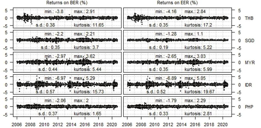
Jetsada LAIPAPORN, Phattrawan TONGKUMCHUM /
2                                 Journal of Asian Finance, Economics and Business Vol 8 No 3 (2021) 0001–0010

(ASEAN) set up an initiative to establish a free trade area            to statistical formulas or statistical models (Laipaporn &
in order to eliminate trade barriers and support regional              Tongkumchum, 2017). A spline is a function that many
integration (Ahmed & Singh, 2016). Consequently, the                   studies have employed to estimate volatility because its
blueprint of the ASEAN community has been declared as a                continuous piece-wise polynomials are flexible to capture
masterplan to establish a single market of goods and services          the cyclical pattern of financial volatility. The Spline
as well as capitals and skilled labors (Ponziani, 2019; Rillo,         Generalized Autoregressive Conditional Heteroscedasticity
2018). Since then, ASEAN has become a safety area against              or Spline-GARCH model introduced by Engel and Rangel
sudden capital outflow (Harvey, 2017) and more attractive to           (2008) and the Generalized Autoregressive Conditional
foreign direct investment, especially the ASEAN-5 countries            Heteroscedasticity Mixed Data Sampling or GARCH-
including Thailand, Singapore, Malaysia, Indonesia, and the            MIDAS model proposed by Engle, Ghysels and Sohn (2013)
Philippines (Tri, Nga, & Duong, 2019).                                 are examples of volatility model that utilizes spline function.
     The financial infrastructure of the ASEAN-5 economy has           They used the spline function in a quadratic polynomial
been steadily changing over the past fifteen years. Moreover,          form as a part of their model to capture the dynamics of
after the global financial crisis, the US dollar became less           low-frequency volatility and investigate the relationship
stable (Gavranic & Miletic, 2016) and caused instability in            between low-frequency volatility and macroeconomic
the world’s monetary system (Staszczak, 2015). This situation          variables.
possibly affected the exchange rate volatility of the ASEAN-5              Similarly, the NCSV model also utilizes a natural cubic
currencies. Therefore, this study aims to apply the natural            spline function to estimate financial volatility. A natural
cubic spline volatility model to explore the dynamic patterns          cubic spline function is another functional form of a spline,
of the exchange rate volatilities of the ASEAN-5 currencies            which is piecewise cubic polynomials that are linear
both in terms of the bilateral exchange rates and the effective        beyond the extreme knots (Laipaporn & Tongkumchum,
exchange rates from January 2006 to August 2020.                       2017). Recently, Laipaporn and Tongkumchum (2020)
     The natural cubic spline volatility or NCSV model has             employed the NCSV model to estimate the volatilities
been proposed in the study of Laipaporn and Tongkumchum                of the ASEAN-5 stock index and used these estimated
(2017). Though, this model is practical to reveal the                  volatilities to construct the time-varying correlations in
dynamic patterns of the estimated volatility (Farida,                  order to illustrate the patterns of co-movement among
Makaje, Tongkumchum, Phonon, & Laipaporn, 2018),                       ASEAN-5 stock market index. Likewise, Farida, Makaje,
it still needs to identify an appropriate number of knots in           Tongkumchum, Phon-on, and Laipaporn (2018) also
order to influence the model’s goodness of fit (Laipaporn &            applied the NCSV model to estimate the volatility of crude
Tongkumchum, 2018).                                                    oil price. The study found a cyclical pattern of the volatility
     Previous studies have usually applied a user-specified            dynamics identical to the pattern obtained by the other
number of knots to the NCSV model. However, in this                    volatility model.
study, the Monte Carlo simulation will be used to find                     However, one critical issue of utilizing spline function
a proper data-driven criterion to select a number of                   for volatility modeling lies in knot selection. Knots are the
knots among candidate criteria, including the Akaike’s                 connectors between the continuous piece-wise polynomials
Information Criteria (AIC), Bayesian Information Criteria              of the spline function. The flexibility of the spline function
(BIC), General Cross-Validation (GCV), and Modified                    depends on the number of knots used to compile the function.
General Cross-Validation (MGCV), and then employ the                   Consequently, an excessive number of knots might lead to an
most appropriate criterion to specify the number of knots              over-fitted volatility model, on the other hand, an inadequate
of the NCSV model for estimating the ASEAN-5 exchange                  number of knots tends to provide the under-fitted model
rate volatilities.                                                     (Laipaporn & Tongkumchum, 2018). Additionally, a spline
     The remainder of this article is organized as follows.            function with many knots is not guaranteed to provide a
Section 2 and section 3 present the background and details             more fitted model (Breiman, 1993).
of the methodology used in this study. The simulation results              Laipaporn and Tongkumchum (2020) and Farida et al.
on the knot selection criteria and the empirical results on            (2018) applied a user-specified number of knots in their
the ASEAN-5 exchange rates’ volatilities are stated and                respective studies. They subjectively selected an appropriate
discussed in Section 4. The conclusions made from this                 number of knots concerning the data investigated in their
study are presented in Section 5.                                      studies. By applying the equi-spaced knots, Laipaporn and
                                                                       Tongkumchum (2020) set an interval between knots at
2. Literature Review                                                   250 trading-day per interval and then assigned a number of
                                                                       knots according to that interval and a number of observations.
    Volatility is not directly measured like weight and height         Likewise, Farida et al. (2018) set the length between knots
but it is usually calculated or estimated from its proxy, returns      at almost 200 trading-days and consequently determined the
on the financial asset’s price or financial index, according           number of knots for their NCSV model.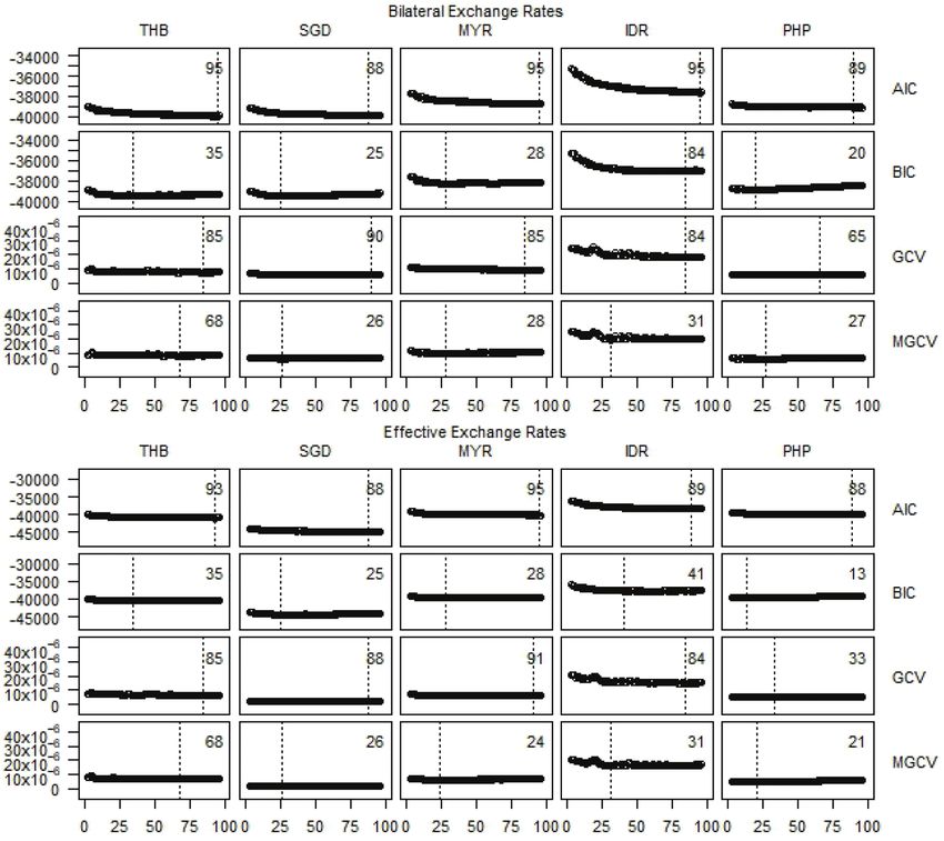
Jetsada LAIPAPORN, Phattrawan TONGKUMCHUM /
Journal of Asian Finance, Economics and Business Vol 8 No 3 (2021) 0001–0010 3
In contrast, previous studies that used the spline-GARCH rt = n(0, σt)(1)
model and the GARCH-MIDAS model alternatively
determined the number of knots by utilizing information Ten types of pre-specified volatilities were determined
criteria such as Akaike’s Information Criteria (AIC) and as the rolling standard deviation of the daily returns of
Bayesian Information Criteria (BIC) (Conrad & Kleen, ASEAN-5 bilateral exchange rates with two different rolling
2020; Lee, Stevenson, & Lee, 2018; Engle, Ghysels, & windows which are 60 and 120 trading days per window.
Sohn, 2013; Engle & Rangel, 2008). Note that the wider rolling windows provide less fluctuated
Similarly, Laipaporn, and Tongkumchum (2018) also rolling standard deviations.
employed both the AIC and BIC criteria for selecting a Based on ten types of pre-specified volatility, ten
number of knots for the NCSV model. They found that AIC groups of 500 series of 1,500 simulated daily returns were
performed well to the simulated dataset but failed to provide generated and used as a dataset used for the Monte-Carlo
the appropriate knots for the NCSV model in the case of the simulation. An example of simulated returns series in
empirical data. However, the number of equi-spaced knots absolute term and its corresponding pre-specified volatility
using in Laipaporn and Tongkumchum (2018) is exponentially are shown in Figure 1.
increasing by 2n−1 where n is an increasing step. This procedure As introduced in Laipaporn and Tongkumchum (2017),
is different from the other studies, which usually increase the the NCSV model is based on the assumption that the
number of knots one at a time. time series of the financial returns (rt) is the product of
Based on prior studies, there are other approaches that time-varying volatility (st) and random noise (εt), which is
have been used to determine the number of knots in a spline normal distributed with a zero mean and a unit standard
function. Montoya, Ulloa, and Miller (2014) compared deviation as follows.
various knots selection criteria and found that generalized
cross-validation or GCV introduced by Craven and Wabha rt st
t (2)
(1979) is more suitable method in selecting the number of
knots for the penalized regression spline model. Likewise,
Chen, Abraham, and Bennett (1997) and Lewis and Stevens The time-varying volatility (st) is parameterized as the
(1991) utilized the modified generalized cross-validation natural cubic spline function with respect to time (t = 1, 2,
or MGCV proposed by Friedman (1991) for selecting the 3, …, T ) as the succeeding equation.
number of knots of the multivariate adaptive regression or
MARS model. They found that this approach provided a t p
tk 3
parsimonious time series model that exhibited a cyclical p
2
t
tk
3
t
t
t
t p
1
st
t
k
p p
1
pattern of the time series data. (3)
t
t
Hence, this study investigates more candidate criteria other
p
1 k
t
t p
k 1
3
than the AIC and BIC to find the most appropriate approach t p
t p
1
for modeling the NCSV model and alternatively increasing the
number of quantile knots of the NCSV model one at a time. The total number of observations is equal to T, p is
a number of knots k where k = 1, 2, 3, …, p. Each knot
3. Research Methods and Materials is placed at tk which is a quantile order k of time t in the
interval [1, T].
Two dataset were used in this study. The first dataset is To estimate the parameters of the NCSV model, the
the daily returns of the ASEAN-5 bilateral exchange rates natural cubic spline function is applied to the absolute values
and their effective exchange rates from January 2006 to of the returns series (|rt|), which are the proxies of the daily
August 2020. The daily returns series are the logarithm returns volatility (Figlewski, 1997). Consequently, the parameters of
calculated using their corresponding exchange rates, which this function (α, β and θk) are estimated by maximizing the
were retrieved from the website of Bank of International log-likelihood function (L) as follows.
Settlements. They comprised of the exchange rates of Thai
baht (THB), Singapore dollar (SGD), Malaysian ringgit
rt
2
T
(MYR), Indonesian rupiah (IDR), and Philippine peso (PHP). L
log
st
(4)
The second dataset is the simulated returns series. it is t 1 2 st2
generated for the Monte Carlo simulation in order to find a
proper criterion to select an appropriate number of knots for This study set three steps to select the NCSV model
the NCSV model. By supposing that true volatility is known, with the optimal number of knot based on previous
this study generated the simulated daily returns series as a literature works. The first step is to determine a possible
random noise with zero mean and pre-specified volatility (σt) range of a number of knots p. A number of knots p usually
using the following equation. begins with three as the lower limit of the possible range.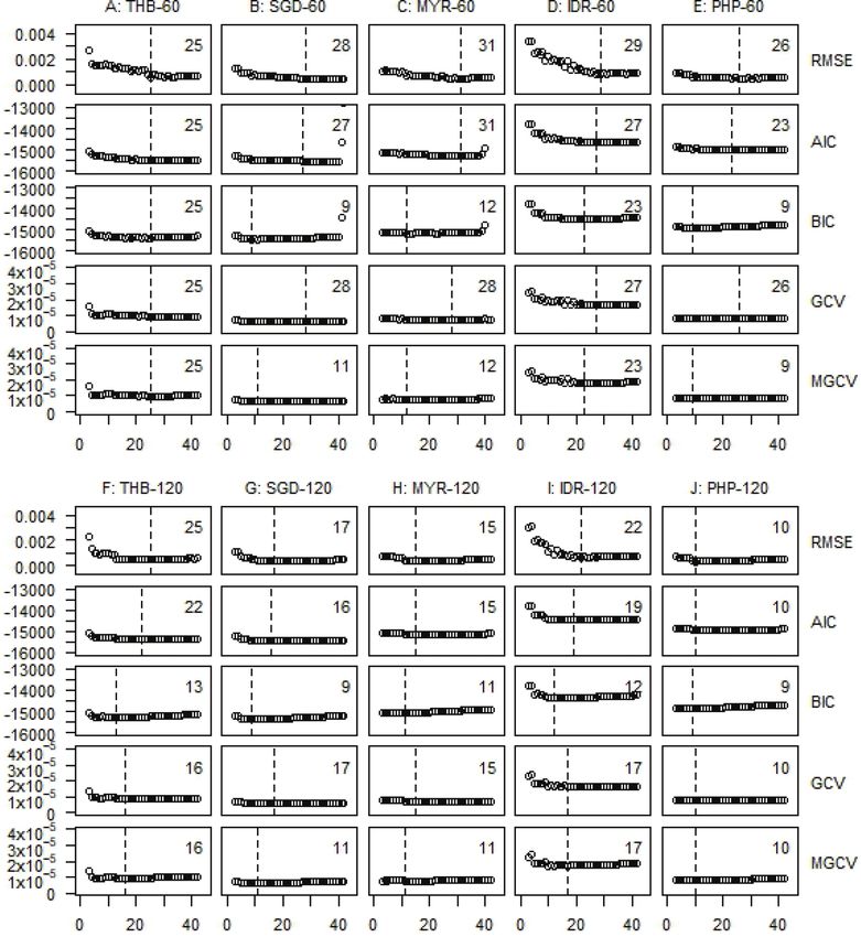
Jetsada LAIPAPORN, Phattrawan TONGKUMCHUM /
4                                      Journal of Asian Finance, Economics and Business Vol 8 No 3 (2021) 0001–0010

                             Figure 1: Examples of Simulated Daily Returns in Absolute Term and
                                        their Corresponding Pre-Specified Volatilities

The three knots include two boundary knots at the first and the                 Note that d in the MGCV formula is a parameter
last observation and one interior knot in the middle. To ensure             representing the cost of the increased knot in the spline
that there are at least 40 observations which is the number                 function. The larger number of d tends to signify a fewer
of observations in one quarter between each knot. The upper                 number of knots. This study sets d equal to 2 following the
limit of the number of knots is therefore set at T p < 40 .                 recommendation in Friedman (1991). The NCSV model
    The second step is to estimate the NCSV model’s                         with the least value of each criterion, consequently indicates
parameters with the number of knots in the possible range.                  the optimal number of knots for that criterion.
The third step is to apply four candidate criteria: AIC, BIC,                   For the simulated return datasets, the root mean square
GCV and MGCV to the NCSV model obtained from the                            error (RMSE) of the pre-specified volatility (σt) and the
second step using the following formula.                                    estimated volatility (st) estimated by the NCSV model is
                                                                            calculated as the following equation.
                   AIC   L  2 p (5)
                   BIC   L  p log  n  (6)                                                                 t  st
                                                                                                                             2

                                                                                                  RMSE                          (9)
                                                                                                                      T
                               T
                          T 1   rt  st
                                                  2

                                                                                The NCSV model with the least RMSE indicates the
                  GCV         t 1
                                                      (7)
                             p  1
                                              2
                                                                            optimal number of knot corresponding to each pre-specified
                           1                                             volatility. Accordingly, this optimal number became the
                               T                                          benchmark number of knots for the performance comparison
                                   T                                        among four criteria in the Monte Carlo simulation.
                            T 1   rt  st
                                                      2
                                                                            A candidate criterion that specifies the number of knots
                MGCV              t 1
                                                              (8)          closest to the benchmark number is the most appropriate
                            p  1  dp
                                                          2
                                                                            knot selection criterion for estimating the NCSV model of
                          1
                                 T                                        the ASEAN-5 currencies.
Jetsada LAIPAPORN, Phattrawan TONGKUMCHUM /
                            Journal of Asian Finance, Economics and Business Vol 8 No 3 (2021) 0001–0010                         5

4. Results and Discussion                                                  According to each criterion, the vertical line and the
                                                                       number at the corner of each graph indicate the least
    For the Monte Carlo simulation, the simulated returns              averages and an optimal number of knots. The least
series according to ten types of pre-specified volatilities were       average values of RMSE specify the benchmark number
applied to the NCSV model with a number of knots in the                of knots for each group of simulated returns. The first five
possible range varying from 3 to 42 knots. Since each returns          groups of simulated returns were generated by 60 trading
series has 1,500 observations, the interval size between knots         days rolling standard deviation (A, B, C, D, E), mostly
of the NCSV model thus varies from nearly 40 observations              require more number of knots for the NCSV model than
to 750 observations per interval.                                      the simulated returns generated by 120 trading days rolling
    Figure 2 shows graphs plotting the number of knots in              standard deviation (F, G, H, I, J). It implies that if true
the possible range and the averages of RMSE, AIC, BIC,                 volatility is high fluctuated, it will require more knots to
GCV and MGCV obtained from the NCSV models.                            model the NCSV.

    Figure 2: The Number of Knots and the Average Values of RMSE, AIC, BIC, GCV and MGCV from the NCSV Models
                                        by Ten Groups of the Simulated Returns
Jetsada LAIPAPORN, Phattrawan TONGKUMCHUM /
6 Journal of Asian Finance, Economics and Business Vol 8 No 3 (2021) 0001–0010
Regarding the benchmark number, a proper knot at a time. This contrasts with Laipaporn and Tongkumchum
selection criterion has to select neither too many nor too few (2018) study where an increase in the number of knots
numbers of knots than the benchmark number. Among the occurred exponentially from 3 to 7, 15, 31, 63, 127, etc.
ten groups of simulated returns, GCV selects the number of Although increasing the number of knots one at a time is a
knot identical to the benchmark number for six groups (A, B, time-consuming process, this simulation demonstrates that
E, G, H, J). For the other four groups (C, D, F, G), GCV this approach is entirely accurate in determining the number
selects a less number of knots, but it is not much different of knots for the NCSV model.
from the benchmark. Likewise, AIC selects the number of For the empirical part, the series of 3,773 daily
knot identical to the benchmark for four groups of simulated returns on the bilateral exchange rates and the effective
returns (A, C, H, J). exchange rates of the ASEAN-5 currencies are presented
In contrast, there is only one group of simulated returns in Figure 3.
(A) that BIC identifies the number of knots identical the Mean values of these daily returns series are tested and
benchmark number. For the rest groups, the number of knot they are not significantly different from zero. Among the
indicated by BIC is much less to the benchmark number. five currencies, IDR has the broadest range of daily returns
MGCV is a little better than the BIC. It selects the same series. The differences between the minimum and maximum
number of knots as the benchmark number for two groups of value of its bilateral and effective exchange rates are nearly
simulated returns (A, J). The BIC and MGCV do not perform 13 and 12 percentage points, respectively. These two series
well for the groups of simulated returns with more fluctuated also have the highest kurtosis at 15.7 and 19.7 points.
pre-specified volatility (60 trading days rolling standard Whereas, SGD has less varied daily returns series than the
deviation). However, they tend to select a number nearer to others. The standard deviations of its bilateral and effective
the benchmark for the groups of simulated returns generated exchange rates are 0.35 and 0.19, respectively. The skewness
by less fluctuated pre-specified volatility (120 trading days of all series is relatively small. They are close to zero in the
rolling standard deviation). range between −0.61 and 0.28.
Following the simulation results, GCV is the most To determine the proper NCSV models of ASEAN-5
preferred criterion, while the second-best criterion is the exchange rates, a set of pre-specified number knots is
AIC. In contrast, the BIC provides a small number of knots assigned from 3 to 96. The size of the interval between knots
for most cases. This result is similar to Laipaporn and varies from nearly 40 observations to 1,886 observations
Tongkumchum (2018), which found the AIC to be a more per interval. The values of AIC, BIC, GCV and MGCV of
preferred criterion than the BIC in the case of simulated data. the NCSV models of the ASEAN-5 exchange rates and the
Note that the number of knots in this study increases one possible range number of knots are displayed in Figure 4.
Figure 3: Returns on the Bilateral Exchange Rates (BER) and
the Effective Exchange Rates (EER) of the ASEAN-5 CurrenciesJetsada LAIPAPORN, Phattrawan TONGKUMCHUM /
Journal of Asian Finance, Economics and Business Vol 8 No 3 (2021) 0001–0010 7
Figure 4: The AIC, BIC, GCV and MGCV from the NCSV Models of
Daily Returns of ASEAN-5 Currencies Currencies
The number of knots for the NCSV models of ASEAN-5 Since the effective exchange rates are less volatile, in
exchange rates indicated by BIC is relatively fewer than some cases GCV designates a smaller number of knots than
the number obtained by the other three criteria. Likewise, a number of knots of the bilateral exchange rates’ volatility
MGCV often selects a number of knots identical to a number models. The intervals between knots according to the number
chosen by BIC. Therefore, BIC and MGCV tend to indicate of knots selected by GCV in this study vary from 42 to 118
an under-fitted model. GCV and AIC select an equivalent trading days. These intervals are much smaller than the
number of knots in some cases. However, the behavior in intervals assigned by the same criterion in Engle and Rangel
knot selection of GCV is more consistent than AIC, because (2008) for the volatilities of the ASEAN-5 stock index. Note
in some cases, AIC assigns too large number of knots for that the functional form of the spline function used in this
the NCSV model. Regarding this comparison, the GCV is study is a natural cubic spline function, which is different
likely to provide an accurate number of knots for modeling from the quadratic spline function used in Engle and Rangel
the natural cubic volatility of the ASEAN-5 exchange rates. (2008). The natural cubic spline is more flexible than theJetsada LAIPAPORN, Phattrawan TONGKUMCHUM /
8 Journal of Asian Finance, Economics and Business Vol 8 No 3 (2021) 0001–0010
quadratic spline. Consequently, it needs a more number of The exchange rate volatilities of THB were more than
knots to fit the volatility model. 10 percent in that period, and then diminished to less than
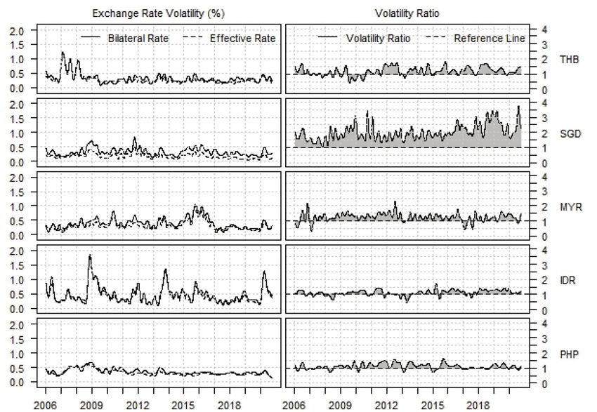
The volatilities of ASEAN-5 exchange rates estimated 5 percent after the crisis. This shows the exchange rate
by the natural cubic spline volatility models with a number of THB is stable after the global crisis until now. The
of knots selected by GCV are shown in Figure 5. Graphs exchange rates of MYR are less stable between 2015 to
in the left column illustrate the comparison of the bilateral 2016 since the MYR depreciation to the world currencies
exchange rate volatilities (BER) and the effective exchange in October 2015 (Quadry, Mohamad, & Yusof, 2017).
rate volatilities (EER) of the ASEAN-5 currencies in the same Malaysia increases their money supply by lowering its
axis, while graphs in the right column show the volatility interest rate to absorb the exchange rate shock (Kaur,
ratio, the ratio of the bilateral exchange rate volatilities over Manual, & Eeswaran, 2019).
the effective exchange rate volatilities of the corresponding The reference lines in the left graphs of Figure 5 indicates
currencies. the volatility ratio equal to one. As shown in Figure 5, in
The dynamic patterns of the bilateral exchange rate the period that the exchange rate volatility ratios of the
volatility of the ASEAN-5 currencies are not entirely different ASEAN-5 currencies are higher than the reference line,
from the pattern of the same currencies’ effective exchange rate the bilateral exchange rates of the ASEAN-5 currencies
volatility. The bilateral and effective exchange rate of IDR is are more volatile than its corresponding effective exchange
more volatile than the other currencies, while the exchange rate rates. The volatility ratios of the ASEAN-5 currencies are
volatilities of SGD and PHP indicate that these two currencies mostly higher than the reference line, especially SGD; its
are more stable than the other currencies. The finding is similar bilateral exchange rate volatility is almost twice higher than
to Ponziani (2019) and Klyuev and Dao (2017). its effective exchange rate volatility. The average volatility
The bilateral and effective exchange rates of THB are ratios of THB, SGD, MYR, IDR and PHP are 1.17, 1.99,
most volatile during the global financial crisis period. 1.24, 1.12 and 1.11 respectively.
Figure 5: The Estimated Volatilities and the Volatility Ratios of the
ASEAN-5 Bilateral and Effective Exchange RateJetsada LAIPAPORN, Phattrawan TONGKUMCHUM /
Journal of Asian Finance, Economics and Business Vol 8 No 3 (2021) 0001–0010 9
Since the stability of the effective exchange rate ebscohost.com/login.aspx?direct=true&db=bth&AN=1153184
reflects its typical characteristic, which can absorb the 12&site=ehost-live
uncertain exchange rate policies of its trade partners (Thuy Al-Abri, A., & Baghestani, H. (2015). Foreign investment and real
& Thuy, 2019), the SGD was more capable to confront the exchange rate volatility in emerging Asian countries. Journal
uncertainty in the international trade and investment than of Asian Economics, 37, 34–47. https://doi.org/10.1016/j.
the other currencies. This is because the stability of the US asieco.2015.01.005
dollar affects the volatility of the bilateral exchange rates. Breiman, L. (1993). Fitting additive models to regression data:
Several studies are likely to eliminate the influence of the US Diagnostics and alternative views. Computational Statistics
dollar instability by employing the effective exchange rate & Data Analysis, 15, 13–46. https://doi.org/10.1016/0167-
volatility rather than the bilateral exchange rate volatility 9473(93)90217-H
in order to examine the real stability of the currency (Kaur, Campa, A. C. Jr. (2020). Capturing the short-run and long-run
Manual, & Eeswaran, 2019; Thuy & Thuy, 2019; Al-Abri & causal behavior of Philippine stock market volatility under
Baghestani, 2015). vector error correction environment. Journal of Asian Finance,
Economics and Business, 7(8), 41–49. https://doi.org/10.13106/
jafeb.2020.vol7.no8.041
5. Conclusions
Chen, G., Abraham, B., & Bennett, G. W. (1997). Parametric and
To estimate the exchange rate volatility of the ASEAN-5 non-parametric modelling of time series: An empirical study.
currencies, this study applied the natural cubic spline model Environmetrics, 8, 63–74. https://doi.org/10.1002/(SICI)1099-
095X(199701)8:13.0.CO;2-B
with various data-driven knot selection criteria comprised
of the AIC, BIC, GCV and MGCV. This study further Conrad, C., & Kleen, O. (2020). Two are better than one: Volatility
employed the Monte Carlo simulation to find the most forecasting using multiplicative component GARCH-MIDAS
appropriate knot selection criteria. The simulation showed models. Journal of Applied Econometrics, 35(1), 19–45. https://
doi.org/10.1002/jae.2742
that GCV is the most preferred since it assigns a number of
knots closest to the benchmark number. The BIC and MGCV Craven, P., & Wabha, G. (1979). Smoothing noisy data with spline
tend to determine a smaller number than the other criteria in functions: Estimating the correct degree of smoothing by method
simulated datasets and empirical datasets. For the simulated of generalized cross-validation. Numerische Mathematik,
31(4), 377–403. https://doi.org//10.1007/BF01404567
dataset, AIC performs well. It often selects an identical
number of knot to the benchmark knots. However, it selects Dang, V. C., Le, T. L., Nguyen, Q. K., & Tran, D. Q. (2020). Linkage
too much number of knots for the empirical datasets. between exchange rate and stock prices: Evidence from Vietnam.
Additionally, the exchange rate volatilities of the Journal of Asian Finance, Economics and Business. 7(12),
95–107. https://doi.org/10.13106/jafeb.2020.vol7.no12.095
ASEAN-5 currencies, estimated using the natural cubic
spline model with a number of knots selected by GCV, Engle, R. F., & Rangel, J. G. (2008). The spline-GARCH model
revealed the inconstant dynamic pattern of the ASEAN-5 for low-frequency volatility and its global macroeconomic
exchange rate volatilities. The effective exchange rates causes. The Review of Financial Studies, 21(3), 1187–1222.
Retrieved November 1, 2020 from: https://www.jstor.org/
of the ASEAN-5 currencies have less variation than the
stable/40056848
bilateral exchange rates, especially the bilateral exchange
rate of the Singapore dollar, which is almost twice larger Engle, R. F., Ghysels, E., & Sohn, B. (2013). Stock market volatility
than the effective rate. It is clear evidence showing the and macroeconomic fundamentals. The Review of Economics and
Statistics, 95(3), 776–797. https://doi.org/10.1162/REST_a_00300
stability of the Singapore dollar and the influence of the US
dollar on the variation of the bilateral exchange rate of the Farida, Makaje, N., Tongkumchum, P., Phon-on, A., & Laipaporn, J.
ASEAN-5 currencies. (2018). Natural cubic spline model for estimating volatility.
International Journal on Advanced Science, Engineering
and Information Technology, 4(8), 1085–1090. https://doi.
References org/10.18517/ijaseit.8.4.3107
AbuDalu, A., Ahmed, E. M., Almasaled, S. W., & Elgazoli, A. I. Figlewski, S. (1997). Forecasting volatility. Financial Markets
(2014). The real effective exchange rate impact on ASEAN-5 Institutions and Instruments, 6(1), 1–88. https://doi.org/10.
economic growth. International Journal of Economics & 1111/1468-0416.00009
Management Sciences, 3(2), 1–11. https://doi.org/10.4172/2162- Friedman, J. H. (1991). Multivariate adaptive regression splines.
6359.1000174 The Annals of Statistics, 19(1), 1–67. https://doi.org/ 10.1214/
Ahmed, F., & Singh, V. K. (2016). Financial integration among aos/1176347963
RCEP (ASEAN+6) economies: Evidences from stock and Gavranic, K., & Miletic, D. (2016). US dollar stability and the global
forex markets. South Asian Journal of Management, 23(1), currency reserves. Eurasian Journal of Economics and Finance,
164–188. Retrieved November 1, 2020 from: http://search. 4(3), 14–24. https://doi.org/10.15604/ejef.2016.04.03.002Jetsada LAIPAPORN, Phattrawan TONGKUMCHUM /
10 Journal of Asian Finance, Economics and Business Vol 8 No 3 (2021) 0001–0010
Harvey, B. (2017). Evaluating financial integration and cooperation Business and Accountancy Ventura, 22(2), 283–297. https://
in the ASEAN. Michigan Business & Entrepreneurial Law doi.org/10.14414/jebav. v22i2.1912
Review, 7(1), 119–158. Retrieved November 1, 2020, from: Purwono, R., Mucha, K., & Mubin, M. K. (2018). The dynamic of
https://repository.law.umich.edu/cgi/viewcontent.cgi?article= Indonesia’s current account deficit: Analysis of the impact of
1067&context=mbelr exchange rate volatility. Journal of Asian Finance, Economics
Kaur, T. A., Manual, V., & Eeswaran, M. (2019). The volatility of and Business, 5(2), 25–33. https://doi.org/10.13106/jafeb.2018.
the Malaysian ringgit: Analyzing its impact on economic growth. vol5.no2.25
International Journal of Recent Technology and Engineering, Quadry, M. O., Mohamad, A., & Yusof, Y. (2017). On the Malaysian
7(5S), 82–88. Retrieved November 1, 2020, from: https://www. ringgit exchange rate determination and recent depreciation.
ijrte.org/wp-content/uploads/papers/v7i5s/Es212901751919.pdf International Journal of Economics, Management and
Kennedy, K., & Nourzad, F. (2016). Exchange rate volatility and Accounting, 25(1), 1–26. Retrieved November 1, 2020 from:
its effect on stock market volatility. International Journal of https://journals.iium.edu.my/enmjournal/index.php/enmj/article/
Human Capital in Urban Management, 1(1), 37–46. https:// view/366
doi.org/10.7508/ijhcum.2016.01.005 Rillo, A. D. (2018). ASEAN financial integration: Opportunities,
Klyuev, V., & Dao, T.-N. (2017). No more clubbing, the evolution risks and challenges. Public Policy Review, 14(5), 901–923.
of exchange rate behaviour in the ASEAN-5 countries. Journal Retrieved November 1, 2020, from: https://www.mof.go.jp/
of Southeast Asian Economies, 34(2), 233–265. https://doi. english/pri/publication/pp_review/ppr14_05_04.pdf
org/10.1355/ae34-2a Singh, V. K., & Ahmed, F. (2016). Econometric analysis of
Laipaporn, J., & Tongkumchum, P. (2017). Maximum likelihood financial co-integration of least developed countries (LDCS)
estimation of non-stationary variance. In: Proceedings of of Asia and the Pacific. China Finance Review International,
International Statistical Institue Regional Statistics Conference 6(2), 208–227. https://doi.org/10.1108/CFRI-06-2015-0056
2017 (ISI RSC 2017), (pp. 774–780). Bali. Soleymani, A., Chua, S. Y., & Hamat, A. C. (2017). Exchange rate
Laipaporn, J., & Tongkumchum, P. (2018). The use of information volatility and ASEAN-4’s trade flows: is there a third country
criteria for selecting number of knots in natural cubic effect?, International Economics and Economic Policy, 14,
spline volatility estimation. In Proceedings of International 91–117. https://doi.org/10.1007/s10368-015-0328-9
Conference of Applied Statistics 2018 (pp. 161–164). Bangkok: Staszczak, D. E. (2015). Global instability of currencies: reasons
Faculty of Sciences and Technologies, Prince of Songkla and perspectives according to the state-corporation hegemonic
University, Pattani campus. stability theory. Revista de Economia Politica, 35(1), 174–198.
Laipaporn, J., & Tongkumchum, P. (2020). The time-varying https://doi.org/10.1590/0101-31572015v35n01a10
correlation estimator using the natural cubic spline volatility. Tan, K. G., Duong, L. N., & Chuah, H. Y. (2019). Impact of
Advances and Applications in Statistics, 62(1), 79–95. http:// exchange rates on ASEAN’s trade in the era of global value
doi.org/10.17654/AS062010079 chains: An empirical assessment. Journal of International
Lee, C. L., Stevenson, S., & Lee, M. -L. (2018). Low-frequency Trade & Economic Development, 28(7), 873–901. https://doi.
volatility of rea estate securities and macroeconomic risk. org/10.1080/09638199.2019.1607532
Accounting and Finance, 58(2018), 311–342. https://doi. Teulon, F., Guesmi, K., & Mankai, S. (2014). Regional stock
org/10.1111/acfi.12288 market integration in Singapore: A multivariate analysis.
Lewis, P. A., & Stevens, J. G. (1991). Nonlinear modeling of time Economic Modelling, 43, 217–224. https://doi.org/10.1016/
series using Multivariate Adaptive Regression Splines (MARS). j.econmod.2014.07.045
Journal of the American Statistical Association, 86(41), Thuy, V. N., & Thuy, D. T. (2019). The impact of exchange rate
864–877. https://doi.org/ 10.1080/01621459.1991.10475126 volatility on exports in Vietnam: A bounds testing approach.
Liu, J., Wang, M., & Sriboonchitta, S. (2019). Examining the Journal of Risk and Financial Management, 12(6), 1–14.
interdependence between the exchange rates of China and https://doi.org/10.3390/jrfm12010006
ASEAN countries: A canonical vine copula approach. Tri, H. T., Nga, V. T., & Duong, V. H. (2019). The determinants
Sustainability, 11, 1–20. https://doi.org/10.3390/su11195487 of foreign direct investment in ASEAN: New evidence from
Montoya, E. L., Ulloa, N., & Miller, V. (2014). A simulation study financial integration factor. Business and Economic Horizons,
comparing knot selection methods with equally spaced knots in a 15(2), 292–303. https://doi.org/10.15208/beh.2019.18
penalized regression spline. International Journal of Statistics and Upadhyaya, K. P., Dhakal, D., & Mixon, F. G. (2020). Exchange
Probability, 3(3), 96–110. https://doi.org/ 10.5539/ijsp.v3n3p96 rate volatility and exports: some new estimates from the
Ponziani, R. M. (2019). Foreign exchange volatility modeling of ASEAN-5. Journal of Developing Areas, 54(1), 65–73. https://
Southeast Asian major economies. Journal of Economics, doi.org/10.1353/jda.2020.0004You can also read