ADAPTIVE CONTROLLER FOR AUTOMATIC MANEUVER OF A
←
→
Page content transcription
If your browser does not render page correctly, please read the page content below
Revista Ibero- Americana de Humanidades, Ciências e Educação- REASE

                                                                                      doi.org/10.29327/217514.7.1-1

          ADAPTIVE CONTROLLER FOR AUTOMATIC MANEUVER OF A
                       SATELLITE DISH RECEIVER

        Controlador adaptativo para manobra automática de um receptor de pratos de satélite

                                         Alvaro Manoel de Souza Soares1
                                             João Bosco Gonçalves2
                                             Paulo Henrique Crippa3

ABSTRACT: The objective is to develop a control system capable of performing the automatic
maneuver of a satellite dish and more accurately with less time maneuvering when compared to
manual maneuver. The dish consists of a study on metal parabola 1.60 m in diameter, two sets
of gears and two electric motors to perform the movements. The physical parameters of the
mechanical system could be easily obtained from a three-dimensional modeling in a CAD
software platform. For modeling the system dynamics we used the similarity of the physical
system under study with an serial manipulator of two degrees of freedom that allowed it to apply
concepts related to kinematics and modeling of robotic manipulators. Through the Denavit-
Hartenberg notation of the direct kinematics of the antenna with two degrees of freedom was
successfully obtained. The dynamic equations describing the motion of the system were raised
through an automatic model implemented in symbolic manipulation software. To that end, an
algorithm that describes the steps necessary to obtain the equations of motion of a robotic
manipulator in open chain, from the Lagrangian method, was developed. A model reference
                                                                                                                      1
adaptive control system was designed and implemented considering the uncertainties of the
model arising from imperfections within the three-dimensional modeling. The results obtained
by simulation of the system of closed loop control were satisfactory as well as the high rates of
the perfect maneuver have been achieved.

Keywords: Serial manipulators. Dynamic equations of motion. Model reference adaptive
control.

RESUMO: O objetivo deste trabalho é o de demonstrar o projeto de um sistema de controle
adaptativo capaz de realizar o apontamento automático de uma antena parabólica de forma mais
precisa e com menor tempo de apontamento quando comparado ao apontamento manual. A
antena parabólica em estudo consta de uma parábola metálica de 1,60 m de diâmetro, dois
conjuntos de engrenagens e dois motores elétricos para realização dos movimentos. Os
parâmetros físicos do sistema mecânico foram facilmente obtidos a partir de uma modelagem
tridimensional em um ambiente CAD. Para a modelagem dinâmica do sistema utilizou-se a
similaridade do sistema físico em estudo com um manipulador de cadeia aberta de dois graus de
liberdade, permitindo aplicar conceitos referentes à cinemática e modelagem de manipuladores

1
  Doutorado em Engenharia Aeronáutica e Mecânica pelo Instituto Tecnológico de Aeronáutica (1997).
Professor assistente da Universidade Estadual Paulista Júlio de Mesquita Filho e Professor assistente
doutor da Universidade de Taubaté. E-mail: alvaro@unitau.br.
2 Doutorado em Engenharia Mecânica, Unicamp, 2004.Professor Adjunto da Universidade Federal do

Espírito Santo. E-mail: joao.b.goncalves@ufes.br.
3 Mestre em Engenharia Mecânica, área de concentração: Automação pela Universidade de Taubaté,

2011.Professor titular da Faculdade Canção Nova. E-mail: eng.paulo@cancaonova.com.

            Revista Ibero-Americana de Humanidades, Ciências e Educação. São Paulo, v.7.n.1, Jan. 2021.
                                             ISSN - 2675 – 3375
Revista Ibero- Americana de Humanidades, Ciências e Educação- REASE

robóticos. Através da notação de Denavit-Hartenberg a cinemática direta da antena com dois graus
de liberdade foi obtida com sucesso. As equações dinâmicas que descrevem o movimento do
sistema foram levantadas através da modelagem automática desenvolvida utilizando-se um
software de manipulação simbólica. Para tanto foi desenvolvido um algoritmo que descreve os
passos necessários para obtenção das equações de movimento de um manipulador robótico em
cadeia aberta, a partir da formulação Lagrangeana. Um sistema de controle adaptativo por modelo
de referência foi projetado e analisado, admitindo-se incertezas do modelo oriundas de
imperfeições contidas na modelagem tridimensional. Os resultados obtidos por simulação do
sistema de controle adaptativo se mostraram satisfatórios e os índices de desempenho esperados
para um perfeito apontamento foram alcançados.

Palavras-chave: Manipuladores robóticos em cadeia aberta. Equações dinâmicas de movimento.
Controle adaptativo por modelo de referência.

INTRODUCTION

        The media play a key role in the development of modern civilization. Many segments
of society use this feature to a rapid and efficient dissemination of information. The satellite has
been used as an effective solution for communication between distant points with each other,
since the existing geostationary satellite coverage reaches kilometer (Ha, T.T., 1986.)
        One of the disadvantages of satellite communications is the manual maneuvering of the
satellite dishes of receipt. Besides being a process of high precision this maneuver demand a long
time, especially when referring to the mobile receiving antennas need to adapt to geographic              2
coordinates and climatic conditions and relief that will be exhibited in each use (Marins,
C.N.M., 2004)
        In this sense many efforts have been applied by telecommunications companies to
improve the maneuver of antennas. The solutions range from systems based on microcontrollers
(Cúnico, M., 2006) until the controllers proportional integrative (PI) and proportional
integrative and derivative (PID) (Queiroz, K.I.P.M., 2006) (Souto, M.C.B., 2009). Classic
modern control systems are presented as the solution to perform the pointing implements
(Armellini, F., 2006) ( Armellini, F., 2010) (Malaquias, I.M., 2009.)
        This paper presents a control system able to perform the automatic appointment a
satellite dish reception in order to minimize the disadvantages found in the manual
maneuvering. Thus, it is accepted for study a parabola antenna made of metal with 1.6 m in
diameter, an iron-based support for attachment to flat surface, and two sets of gears arranged in
a way that enables the movement of the antenna in both directions of displacement: slope and
azimuth. Figure 1 show the schematic of the physical system under study.

            Revista Ibero-Americana de Humanidades, Ciências e Educação. São Paulo, v.7.n.1, Jan. 2021.
                                             ISSN - 2675 – 3375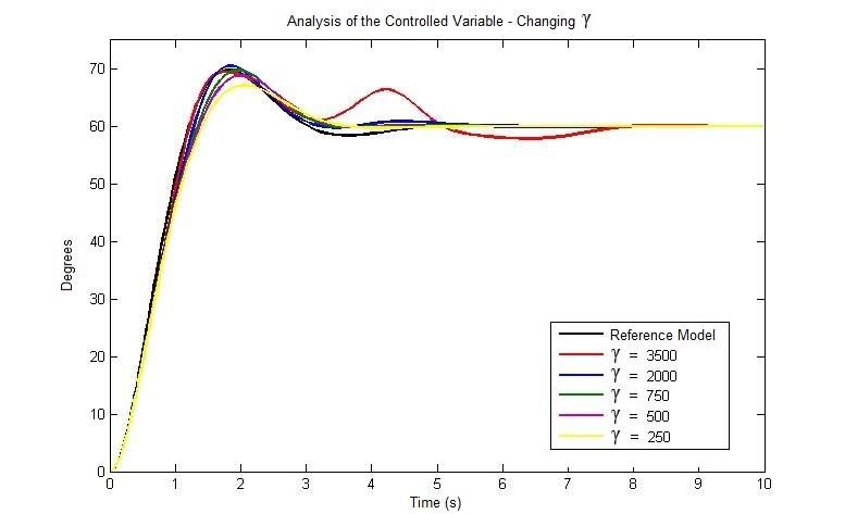
Revista Ibero- Americana de Humanidades, Ciências e Educação- REASE

                                   Fig. 1.   Scheme of Antenna Receiver.

                                                Source: Author.

   The physical system has three rigid links, with a fixed link (link in the base), and two rotary
joints with viscous friction coefficient. Comparing a serial manipulator of the two degrees of
freedom (Schilling, R.J., 1990) (Fu, K., Gonzalez, R.C., Lee C.S.G., 1987) with the physical              3
system under consideration, it is recognized that such a similarity allowed the assignment of the
concepts of kinematics and dynamic modeling of robotic manipulators.
   To develop the control system was used a control action consists of three terms associated
with adaptive control action, a reference model (MRAC) and Computed Torque technique. A
controller MRAC main characteristic is to impose on the system performance indicators in the
reference model. In this work we chose to use an adaptive control action whose unknown
parameters of the plant could be estimated online.
   The analysis of the dynamic behavior of the model obtained, and the control system, took
from its implementation in MATLAB/SIMULINK®.

PHYSICAL SYSTEM SATELLITE RECEIVER

       The prototype of the receiving antenna was designed using the software CATIA® V5
R19 in order to conduct a three-dimensional modeling of the physical system, demonstrating all
the rigid links and rotary joints of the system. The physical parameters of the prototype were
calculated automatically by the software, from the characteristics of materials used, geometric
shapes, dimensions and coordinate systems defined for each hard link.

            Revista Ibero-Americana de Humanidades, Ciências e Educação. São Paulo, v.7.n.1, Jan. 2021.
                                             ISSN - 2675 – 3375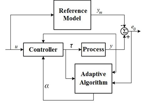
Revista Ibero- Americana de Humanidades, Ciências e Educação- REASE

        The satellite dish receiver consists of rigid links represented by: one support base, one
support for the parables, the parable’s metal, LNB (Low Noise Buffer), and rotary joints along
the rented gear sets.
        The physical system of the receiving antenna was modeled as an articulated system of
rigid links together through the three-dimensional space, which corroborates with the definition
of a robotic serial manipulator [11]. Figure 2 show the result of three-dimensional modeling of
the physical system of the receiving antenna.

                        Fig. 2.   Three-dimensional model of the Antenna Receiver.

                                                                                                          4

                                                Source: Author.

Direct Kinematics

        The software CATIA® V5 R19 allows the inclusion of systems of coordinates in three-
dimensional model [12]. Were assigned the coordinate systems for each link of the physical
model of the receiving antenna following the methodology of Denavit-Hartenberg (DH)
(Adade Filho, A., 1999) (Lopes, A.M., 2002.) Figure 3 shows the result obtained after applying
the procedure DH.

            Revista Ibero-Americana de Humanidades, Ciências e Educação. São Paulo, v.7.n.1, Jan. 2021.
                                             ISSN - 2675 – 3375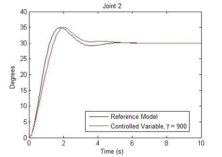
Revista Ibero- Americana de Humanidades, Ciências e Educação- REASE

                                     Fig. 3.     Receiving antenna with DH.

                                                      Source: Author

        The DH parameters of the antenna receiver are shown in Table 1.

                            Table 1. DH parameters of the antenna receiver.
                                                                                                                     5
     Elo(i)              ai (m)                αi (rad)          di (m)             θi (rad)           Variável
       1                  0,19                   -π/2             1,60                 θ1             θ1 (rotação)
       2                  0,97                     0                0                  θ2             θ2 (rotação)

                                                     Source: Author

        With the coordinate systems properly inserted the physical model of the receiving
antenna, CATIA® V5 R19 calculates the moments of inertia and centers of gravity of each rigid
link already referred to the coordinate system attached to the links. Table 2 presents the physical
parameters of three-dimensional model. The moment of inertia for the nth rigid link was
calculated over the n-th Cartesian system, located in the corresponding center of mass. The
crossed moments of inertia are null.

                            Table 2. Physical parameters of the antenna receiver.

              Massa (kg)           Momento de Inércia (kg.m2)                     Centro de Gravidade (m)
  Elo (i)
                 mi                Ix         Iy           Iz                    xc          yc          zc
    1           29,16             58,38      2,09         58,17                -0,14        -1,26       0,07
    2           97,39             7,89      62,40         62,33                -0,76        0,00        0,00

                                                      Source: Author

              Revista Ibero-Americana de Humanidades, Ciências e Educação. São Paulo, v.7.n.1, Jan. 2021.
                                               ISSN - 2675 – 3375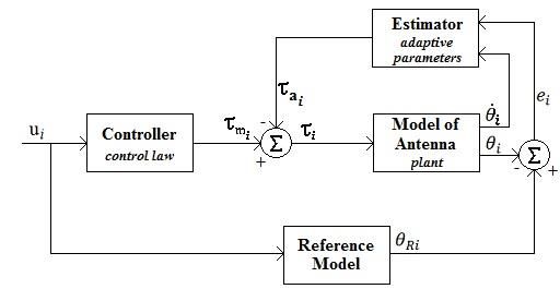
Revista Ibero- Americana de Humanidades, Ciências e Educação- REASE
DYNAMIC MODELING
The purpose of dynamic modeling is to obtain the equations of motion for each degree
of freedom manipulator, allowing relating the movements (displacements) with the generalized
forces (torques) applied at each joint (Latre, L.G., 1988.) According to (Lee, C.S.G.,1983) full
knowledge of the dynamic model of a robot is essential for the computational implementation
of its movement and the control system design.
There are several techniques for dynamic modeling of robotic manipulators (Santos,
R.R., 2005.) Typically the two techniques are widely used in literature to obtain the dynamic
model are the Euler-Lagrange method and the Newton-Euler method. The Newton-Euler
method is to describe the dynamics of a mechanism based on the forces and moments applied to
rigid bodies (links). It is based on two equations: Newton's equation that describes the
translation of the center of mass of rigid body, and the Euler equation that describes the rigid
body rotation around the center of mass. The Euler-Lagrange method is described in a scalar
function of the Lagrangian which is formed by the difference between kinetic energy and
potential energy for each joint system.
The dynamic model of a robotic serial manipulator is expressed by (Santos, R.R., 2005)
n n n
Fi = Dik qk + H ikm q k q m + Ci 6
k =1 k =1 m =1
⑴
In matrix shape:
F (t ) = D(q(t ))q
(t ) + H (q(t ), q (t )) + C(q(t )) . ⑵
where:
F (t ) n x 1 generalized forces vector applied at joints;
D(q(t )) n x n symmetric matrix representing the inertia;
H (q(t ), q (t )) n x 1 nonlinear Coriolis and centrifugal force vector;
C(q(t )) n x 1 gravity loading force vector;
q(t ) n x 1 vector of position of the joint variables;
q (t ) n x 1 vector of velocity of the joint variables;
q(t ) n x 1 vector of acceleration of the joint variables.
Euler-Lagrange method
To determine the dynamic model was used Euler-Lagrange formalism that describes the
dynamic behavior of the system in terms of energy stored in the system (Adade Filho, A., 1999).
The Euler-Lagrange equation is expressed as:
Revista Ibero-Americana de Humanidades, Ciências e Educação. São Paulo, v.7.n.1, Jan. 2021.
ISSN - 2675 – 3375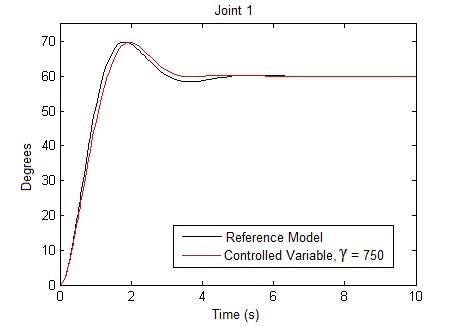
Revista Ibero- Americana de Humanidades, Ciências e Educação- REASE
d L L
− = Fj ⑶
dt q q
j j
Where j is the index related to the rigid element (link), L is the Lagrangian of the system,
given by the difference between kinetic energy and potential energy of the system, and Fj are the
external loads from the potential non-conservative.
Using the Euler-Lagrange equation, the dynamic model of robotic serial manipulator
with rigid links is given by (Fu, K., Gonzalez, R.C., Lee C.S.G., 1987)
i = Tr (U jk J jU )qk + Tr (U jkm J jU Tji )q k q m − m j gU ji j rj
n j n j j n
T
ji ⑷
j =1 k =1 j =1 k =1 m=1 j =1
Comparing Eq. (1) with Eq. (4), are obtained separately the terms of the dynamic
equation of motion:
Tr (U )
n
Dik = jk J jU Tji ⑸
j = max( i ,k )
Tr (U )
n
H ikm = jkm J jU Tji ⑹
j = max( i ,k ,m )
n
7
Ci = − m j gU ji r j j
⑺
j =1
where:
U ji matrix that represents the effects of the motion of joint i on all the points on link
j;
U jkm matrix that represents the interaction effects of the motion of joint k e m on all
the
points on link j;
Jj matrix that contains moments of inertia of link j;
mj mass of link j;
g acceleration of gravity vector referenced to the base coordinate system.
Dynamic Modelo f the Antenna Receiver
To obtain the dynamic model of the satellite dish receiver with two degrees of freedom
will be considered the DH parameters and physical parameters contained, respectively, in Table
1 and Table 2.
Revista Ibero-Americana de Humanidades, Ciências e Educação. São Paulo, v.7.n.1, Jan. 2021.
ISSN - 2675 – 3375Revista Ibero- Americana de Humanidades, Ciências e Educação- REASE
An automatic model was developed using the software Maple ® 13 (Mariani, V.C., 2005)
to implement the Euler-Lagrange formulation developed for a robotic serial manipulator,
described in Eq. (4).
Applying the automatic model was obtained Eqs (8) and (9) that describe the dynamic
model for the physical system of the receiving antenna.
1 = D111 + 2H11212 ⑻
2 = D222 + H 21112 + C2 ⑼
Assuming g = 9.81 m/s2, then the equations will be presented for each term of the
matrices and vectors that describe the dynamic equations of motion. The literal terms contained
therein a1, a2, m1 and m2 respectively, DH parameter of the link 1, parameter DH of the link 2, and
mass of link 1 and mass of link 2. The joints variables are θ1 and θ2 (rotary joints).
Terms of Inertia Matrix Dik :
1 2
D11 = 2a1a2 m2 cos( 2 ) + a1 m1 + a1 m2 + a2 m2 (1 + cos(2 2 )) − 0.29a1m1
2 2
2 ⑽
− 1.514a1m2 cos( 2 ) − 0.757a2 m2 (1 + cos(2 2 )) + 27.2565 cos(2 2 ) + 37.2375
D12 = 0 8
⑾
D21 = 0
⑿
D22 = a2 m2 − 1.514a2 m2 + 62.328
2
⒀
Terms of the vector representing the Coriolis effects and centrifugal force, H ikm :
H 111 = 0 ⒁
1 2
H112 = −a1a2 m2 sin( 2 ) − a2 m2 sin(2 2 ) + 0.757m2 (a1 sin( 2 ) + a2 sin(2 2 ))
2 ⒂
− 27.2565sin(2 2 )
1 2
H121 = −a1a2 m2 sin( 2 ) − a2 m2 sin(2 2 ) + 0.757m2 (a1 sin( 2 ) + a2 sin(2 2 ))
2 ⒃
− 27.2565sin(2 2 )
H 122 = 0 ⒄
Revista Ibero-Americana de Humanidades, Ciências e Educação. São Paulo, v.7.n.1, Jan. 2021.
ISSN - 2675 – 3375Revista Ibero- Americana de Humanidades, Ciências e Educação- REASE
1 2
H 211 = a1a2 m2 sin( 2 ) + a2 m2 sin(2 2 ) − 0.757m2 (a1 sin( 2 ) + a2 sin(2 2 ))
2 ⒅
+ 27.2565sin(2 2 )
H 212 = 0 ⒆
H 221 = 0 ⒇
H 222 =0 ⒇
Terms of the vector representing the effects of gravity acceleration Ci :
C1 = 0 21
C2 = 0.757m2 g cos( 2 ) − m2 a2 g cos( 2 ) 22
The Eqs. (8) e (9) can be placed in matrix shape:
1 D11 0 2 H 112 0 12 0
= 0 +
D22 0
. +
H 211 12 C2
23
2
ADAPTIVE CONTROL SYSTEM
The main objective of a system of closed loop control is to maintain a satisfactory level
of performance even when subjected to disturbances and variations in the control system (Dias, 9
S.M., 2010.)
However, some plants have such wide variations and significant effects on the dynamic
behavior that a classic controller with feedback gain linear and constant coefficients are unable
to provide the necessary flexibility to the system (Tambara, R.V., Gründling, H.A., Della Flora,
L., 2010.)
The basic idea of operation of the adaptive control is to calculate the control signal using
estimates of uncertain parameters of the plant or directly to the controller parameters obtained
through real-time information from the measurable signals of the system (Slotine, J J., Li, W.,
1991.)
Model Reference Adaptive Control (MRAC)
The strategy Model Reference Adaptive Control (MRAC) is considered one of the main
approaches in the literature on adaptive control (Mareels, I.M.Y., Polderman, J.W., 1996.) In
some applications, the plant parameters are not completely known. An alternative to control
solution in these cases is the use of MRAC, where, besides the features of the MRC, the system
inserts a parametric adaptation algorithm which estimates the uncertain parameters of the model
(Tambara, R.V., Gründling, H.A., Della Flora, L., 2010.)
Revista Ibero-Americana de Humanidades, Ciências e Educação. São Paulo, v.7.n.1, Jan. 2021.
ISSN - 2675 – 3375Revista Ibero- Americana de Humanidades, Ciências e Educação- REASE
In the MRAC system performance is expressed in terms of a reference model, which
generates a desired response to a given reference signal. The error between model output and the
output of the plant (eo) is measured, and through methods of parameter estimation (MIT Rule)
controller parameters are modified so that the system behaves like the reference model (Guerra
Vale, M.R.B., Fonseca, D.G.V., Maitelli, A.L., 2008.)
Figure 4 shows the schematic of a MRAC controller.
Fig. 4. Block diagram of a generic MRAC.
Source: Author
Thus, the error between the plant output and the output of the reference model is used 10
to adapt the algorithm to adjust the controller parameters, so that this error tends to zero, thus
allowing the tracking of the asymptotic model (Gonçalves, J.B., 2006.)
MIT Rule
The essential problem of MRAC is to determine the adjustment mechanism so as to
obtain a stable system in which the error signal between the plant output and the output of the
reference model is minimized. The adjustment mechanism called MIT Rule is the original
approach used in MRAC (Bueno, L.P.P., 2006.)
This rule states that for a given error signal e0, a cost function J(α) is calculated, being
α the parameter of the controller to be adjusted. The cost function is defined by:
1 2
J ( ) = e0 24
2
In order to minimize the cost related to the error, the parameter α can be changed
according to the negative gradient of J, so (Ioannou, P., Sun, J., 1995)
Revista Ibero-Americana de Humanidades, Ciências e Educação. São Paulo, v.7.n.1, Jan. 2021.
ISSN - 2675 – 3375Revista Ibero- Americana de Humanidades, Ciências e Educação- REASE
d J e
= − = −e0 0 . 25
dt
The Eq. (26) expresses the MIT Rule. The partial derivative e0 / is called the
derived sensitivity of the system and shows how the error (e0) is influenced by the adjustable
parameter (α). The parameter γ determines the rate of adaptation of the system (adaptive gain).
The mechanism for setting parameters through the MIT Rule is non-linear due to
multiplication of the error with the partial derivative. Application of this mechanism can result
in unstable systems, particularly if the adaptive gain γ is relatively high (Resende, J. M. O. S.
A., 1995.)
MRAC Controller Antenna Receiver
The dynamic model obtained for the physical system of the receiving antenna has a non-
linear as can be seen in Eqs (8) and (9). A linearization technique called Computed Torque was
applied. The purpose of this linearization is to transform all or part of a nonlinear dynamic
system, resulting in a system to which to apply linear control techniques (Slotine, J J., Li, W.,
1991.) 11
The technique MRAC was used in the control design of receiving antenna, in order to
identify the unknown parameters of the plant, so online. Figure 5 shows the block diagram of
the control technique used in automatic maneuvering of the receiving antenna.
Fig. 5. MRAC block diagram of antenna receiver.
Source: Author
Revista Ibero-Americana de Humanidades, Ciências e Educação. São Paulo, v.7.n.1, Jan. 2021.
ISSN - 2675 – 3375Revista Ibero- Americana de Humanidades, Ciências e Educação- REASE
Model Uncertainty
For the design of the control system of the antenna receiver is efficient it is necessary
that the dynamic model is as close as possible to the real physical system. It is assumed that the
term refers to energy dissipation is not known and therefore not included in the equations that
define the dynamic model of the receiving antenna (Eqs. 8 and 9). Therefore the dynamic model
of the receiving antenna must be rewritten with the inclusion of the unknown term energy
dissipative.
Admitting B̂ as the vector that represents the dissipative forces unknown to the model
given by:
bˆ1
ˆ
B= 26
ˆ
b2
The dynamic equations of motion of the antenna receiver can be rewritten as:
1 = D111 + 2 H11212 + bˆ11 27
2 = D222 + H 21112 + C2 + bˆ22 28
In matrix shape:
12
1 D11 0 2 H112 0 12 C1 bˆ1 0 1
= 0 +
D22 0
. + + .
H 211 12 C2 0 bˆ2 2
29
2
Reference Model
For the design of the control system of the receiving antenna was used as a reference
model of a 2nd order system widely discussed in (Nise, N.S., 2009.) Such systems have the well-
defined performance index which allows to easily establish desirable conditions for the plant
output, is in transition and in steady state. Eq. (31) presents the reference model adopted
expressed in the time domain and in the function of natural frequency ωn and damping ratio ζ:
Ri = ni2 ui − 2 niRi − ni2 Ri 30
In matrix shape:
R = Ωu − ZR − Ω R 31
where:
Revista Ibero-Americana de Humanidades, Ciências e Educação. São Paulo, v.7.n.1, Jan. 2021.
ISSN - 2675 – 3375Revista Ibero- Americana de Humanidades, Ciências e Educação- REASE
n21 0
:= 2
0 n2
32
2 0
Z := 1 n1
2 2 n 2
33
0
u
u := 1 34
u 2
R := R1 35
R 2
The natural frequency ωn and damping ratio ζ can be determined from an index of
performance imposed on the closed loop system. In order to perform an automatic pointing of
the antenna receiving satisfactory, it is an overshoot %UP = 15%, and a transient peak time Tp
= 1.8 s.
The relationship between the overshoot %UP and the transient peak time Tp, with the
natural frequency ωn, and damping ratio ζ, are given by:
%UP = e −( / 1− 2 )
36 13
Tp = 37
n 1 − 2
Solving Eqs. (37) and (38), result: ωn = 2 rad/s e ξ = 0.5.
Control law
From the control scheme shown in Figure 5, the adaptive control law used in the antenna
receiver is given by:
i = m + a
i i
38
In order m i
is the term of the model expressed in terms of nominal values obtained in the
dynamic model. Already a i
is the term adaptive expressed as a function of adaptive parameter
to be estimated.
Applying the technique of Computed Torque wishing to eliminate the nonlinearity of the
plant and, considering the uncertain terms of the model bˆ11 and bˆ22 , the terms of the model
control law, m1 and m2 , can be written as:
Revista Ibero-Americana de Humanidades, Ciências e Educação. São Paulo, v.7.n.1, Jan. 2021.
ISSN - 2675 – 3375Revista Ibero- Americana de Humanidades, Ciências e Educação- REASE
m = D11 (Ωu1 − ZR1 − Ω R1 ) + 2 H 11212
1
39
m = D22 (Ωu 2 − ZR 2 − Ω R 2 ) + H 21112 + C 2
2
40
The adaptive terms of the control law, a e a
1 2
, are:
a = 11
1
41
a = 22
2
42
Where, α1 e α2 are the parameters of adaptive control to be set by the estimator.
Therefore, the control law given in Eq. (39) can be rewritten for each degree of freedom
system:
1 = D11 (Ωu1 − ZR1 − Ω R1 )+ 2H11212 + 11 43
2 = D22 (Ωu2 − ZR2 − Ω R2 ) + H 21112 + C2 + 22 44
Estimator – MIT Rule
To estimate the parameters of the adaptive controller was used to MIT rule. In this rule it is
desired that the estimated parameter α converges to α* (optimal value), this implies that
14
lim t → e0 (t ) = 0 , where e0 is the error signal (Guerra Vale, M.R.B., 2008.)
The adaptive parameter of controller is a function of the partial derivative of the plant output
θi with respect to parameter αi multiplied by the error signal. The estimates of the parameters of
the controller can be represented by (Ioannou, P., Sun, J., 1995)
s
1 = − e1 45
s + Zs + Ω
2 1
s
2 = − e 2 46
s + Zs + Ω
2 2
Simulation and results
The implementation of the control system was performed in MATLAB® software
through the toolbox SIMULINK®, which features an intuitive graphical language programming
offering an alternative to the classical approach to numerical simulation of engineering problems
(Matsumoto, É.Y., 2004.)
Revista Ibero-Americana de Humanidades, Ciências e Educação. São Paulo, v.7.n.1, Jan. 2021.
ISSN - 2675 – 3375Revista Ibero- Americana de Humanidades, Ciências e Educação- REASE
In the simulations step functions were used as inputs of the system. Each entry
represents the desired angular displacement for each joint of the system, such that: u1 = 60°, u2 =
30°.
Figure 6 and 7 show the outputs of the plant being controlled by MRAC for the joint 1
and joint 2, respectively, with a fixed gain adaptive (γi) given by: γ1 = 750, γ2 = 900.
Fig. 6. Outputs of the control system – joint 1.
(a) Angular Displacement
(b) Angular Velocity
Fig. 7. Outputs of the control system – joint 2.
15
(d) Angular Velocity
(c) Angular Displacement
Source: Author
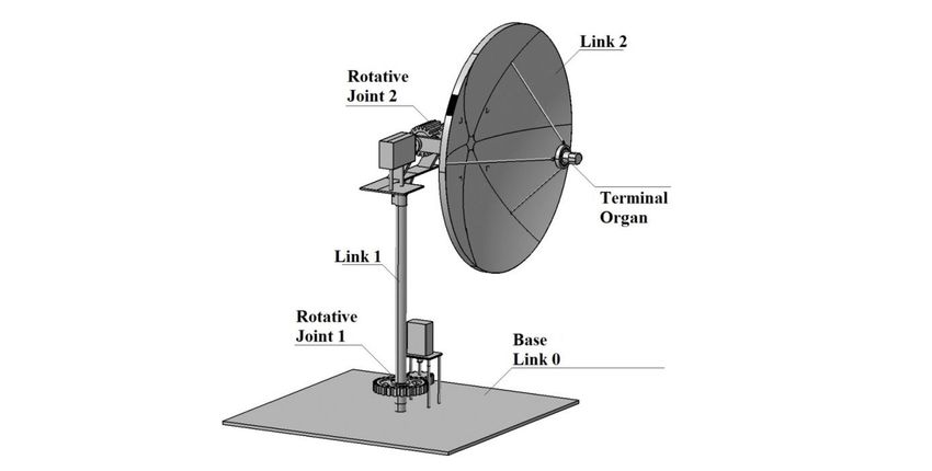
The main characteristic to be observed in an MRAC is the behavior of the controlled
variable relative to the reference model. The latter is chosen so as to impose on the system the
desired levels of performance. Figure 8 shows the output signal (controlled variable) compared
to the reference model adopted.
Fig. 8. Analysis of output signal (controlled variable).
Revista Ibero-Americana de Humanidades, Ciências e Educação. São Paulo, v.7.n.1, Jan. 2021.
ISSN - 2675 – 3375Revista Ibero- Americana de Humanidades, Ciências e Educação- REASE
(a) Controlled Variable – joint 1 (b) Controlled Variable – joint 2
Source: Author
The error signal is obtained by the difference between the reference model and the output
signal of the system. Figure 9 shows the error signal for the joint 1 and 2 of the antenna receiver.
Fig. 9. Error signal.
16
(a) Error Signal of the joint 1 (e1) (b) Error Signal of the joint 2 (e2)
Source: Author
It is observed that the error signals of Figure 9 have small values which show the
effective control action for both joints of the system of antenna receiver.
The model uncertainties are compensated by the parameter adaptive control. For the
purpose of simulation was added to the model with a dissipative term to evaluate the behavior
of parameter adaptive control.
Figure 10 (a) provides for the joint 1, the behavior between the dissipative term inserted
bˆ1
θ1 , and the parameter adaptive control 1 , Figure 10 (b) provides for the joint 2, the
D11
Revista Ibero-Americana de Humanidades, Ciências e Educação. São Paulo, v.7.n.1, Jan. 2021.
ISSN - 2675 – 3375Revista Ibero- Americana de Humanidades, Ciências e Educação- REASE
bˆ2
behavior between the dissipative term inserted θ2 , and the parameter adaptive control
D22
2 . The values of the adaptive gains are set: γ = 750, γ = 900.
1 2
Fig. 10. Analysis of the adaptive controller parameter.
(a) Controller parameter – joint 1 (b) Controller parameter – joint 2
Source: Author
Analyzing Figure 10 shows that the contribution of the dissipative term included in the 17
model rapidly tends to zero (about 5s). This is due to the fact that the velocity also tends to zero
in this short period of time. Satisfactorily the contribution of the adaptive control parameter
influences the system output at the same time interval in which the dissipative term acts. Note
also that the adaptive control parameter tends to zero at the same instant in which the dissipative
term is significant in the system.
The variation of the adaptive gain γ has a direct influence on the behavior of the MRAC.
As the system of the antenna receiver has a fixed gain at its plant the adjusting of the γ occurred
empirically, that is, as varying the γ analyzing the behavior of the output.
Figure 11 and 12 show the influence of γ at the output of a system to seal and joint 2
respectively.
With very high values of γ the systems begin to show features of instability. To perform
the pointing of the antenna receiver with satisfactory levels of play can be considered an adaptive
gain to the joint 1 such that: γ1 ∈ [710, 830] and for joint 2: γ2 ∈ [880, 990].
Revista Ibero-Americana de Humanidades, Ciências e Educação. São Paulo, v.7.n.1, Jan. 2021.
ISSN - 2675 – 3375Revista Ibero- Americana de Humanidades, Ciências e Educação- REASE
Fig. 11. Influence of γ on output system – joint 1.
Source: Author
Fig. 12. Influence of γ on output system – joint 2.
18
Source: Author
CONCLUSION
This work was presented an adaptive control system for the automatic maneuvering of
a receiver dish. For the basis of studies have been adopted the physical and construction
characteristic of a antenna receiver widely used in satellite communications professionals
systems.
The three-dimensional modeling of the physical system made it possible for the antenna
receiver to obtain the physical parameters of the system. This modeling was done in CATIA ®
V5 R19. The features offered by this software enabled the physical model obtained contemplate
Revista Ibero-Americana de Humanidades, Ciências e Educação. São Paulo, v.7.n.1, Jan. 2021.
ISSN - 2675 – 3375Revista Ibero- Americana de Humanidades, Ciências e Educação- REASE
all the constituent parts of the schematic constructive prepared for the mechanism of the antenna
receiver, making it possible to identify the links in the system. The systematic location of
Cartesian coordinate systems in the joints of the system, according to the Denavit-Hartenberg
rules, was also easily performed by this software.
The similarity of the physical system obtained with a robotic serial manipulator allowed
to use the concepts of kinematics and dynamic modeling of manipulators. The Euller-Lagrange
formalism was used in modeling the dynamics of the antenna receiver. To that end, we
developed an algorithm that describes the steps necessary to obtain the dynamic equations of
motion for a robotic serial manipulator. The implementation of this algorithm occurred in the
software MAPLE® 13. As a result of this implementation was developed automatic modeler that
is capable of resulting equations of motion for these manipulators.
The implementation of the MRAC control system adopted to control the movements of
the antenna receiver, took from its implementation in MATLAB® using the toolbox
SIMULINK®.
As the dynamic model obtained was a non-linear model by a feedback linearization
technique (Computed torque) was applied in order to eliminate the nonlinear terms of the
model. The reference model adaptive control action was adopted to control the plant. The
reference model chosen was a standard system of 2nd order, which in addition to the simplicity 19
of implementation allows the desired levels of performance for the system to be easily
established. The parameters of adaptive controller were estimated by MIT rule that evaluates
the sensitivity of the error derivative with respect to the parameter of the controller. The
adaptive gain γ, which determines the rate of adaptation of the system, was adjusted empirically,
drawing upon the expertise of the designer.
Simulations of the control system designed were satisfactory and levels of performance
of the system have been achieved. Were also performed simulations varying the adaptive gain.
It was noticed that for high values of γ the system becomes unstable.
REFERENCES
ADADE FILHO, A. Fundamentos de Robótica: Cinemática, Dinâmica e Controle de
Manipuladores Robóticos. CTA-ITA-IEMP, 1999.
ARMELLINI, F. “Controle Robusto da Antena de um Radar Meteorológico”. XVIII CBA –
Congresso Brasileiro de Automática, 2220-2227 p., 2010.
ARMELLINI, F. Projeto e Implementação do Controle de Posição de Uma Antena de Radar
Meteorológico Através de Servomecanismos. Dissertação de Mestrado – Escola Politécnica da
Universidade de São Paulo /USP, 2006.
Revista Ibero-Americana de Humanidades, Ciências e Educação. São Paulo, v.7.n.1, Jan. 2021.
ISSN - 2675 – 3375Revista Ibero- Americana de Humanidades, Ciências e Educação- REASE
BUENO, L.P.P. Dinâmicas Emergentes na Família de Memórias Associativas Bidirecionais
Caóticas e sua Habilidade para Saltar Passos. Tese de Doutorado – USP São Carlos /
Universidade de São Paulo, 2006.
CÚNICO, M. Posicionamento Automático de Antenas Parabólicas. UnicemP / Centro
Universitário Positivo, 2006.
DIAS, S.M., Controle Adaptativo Robusto Para um Modelo Desacoplado de um Robô Móvel.
Tese de Doutorado – UFRN / Universidade Federal do Rio Grande do Norte, 2010.
DORF, R.C., Bishop, R.H. Sistemas de Controle Modernos. Ed. LTC, 2004.
Fu, K., Gonzalez, R.C., Lee C.S.G. Robotics: Control, Sensing, Vision and Intelligence. Ed.
McGraw-Hill Book Company, 1987.
GONÇALVES, J.B. “A integrated control for a biped walking robot”. RBCM. Journal of the
Brazilian Society of Mechanical Sciences and Engineering, Vol. 28, No. 4, pp. 453–460, 2006.
GUERRA VALE, M.R.B., FONSECA, D.G.V., MAITELLI, A.L., ARAÚJO, F.M.U.,
“Controle Adaptativo por Modelo de Referência Aplicado em Uma Planta de Neutralização de
PH”. INDUSCON – VIII Conferência Internacional de Aplicações Industriais, 2008.
HA, T.T. Digital Satellite Comunications, Macmillan Publishing Comp, USA, 1986.
IOANNOU, P., Sun, J. Robust Adaptive Control. Ed. Prentice Hall, 1995.
LATRE, L.G., “Modelagem e Controle de Posição de Robôs”. SAB. Revista da Sociedade 20
Brasileira de Automática, Vol. 2, No. 1, pp 3-15, 1988.
LEE, C.S.G. “Robot Arm Dynamics”, IEEE Tutorial on Robotics. Computer Society Press, 1983.
LOPES, A.M. Modelação Cinemática e Dinâmica de Manipuladores de Estrutura em Séria.
Dissertação de Mestrado – FEUP / Faculdade de Engenharia da Universidade do Porto, 2002.
MALAQUIAS, I.M. Projeto e Caracterização de um Sistema de Telemetria para Ensaios em
Vôo de Aeronaves Leves. Dissertação de Mestrado – UFMG / Universidade Federal de Minas
Gerais, 2009.
MAREELS, I.M.Y., POLDERMAN, J.W. Adaptive Systems: An Introduction. Ed. Birkhauser,
1996.
MARIANI, V.C. Maple-Fundamentos e Aplicações, Ed. LTC, 2005.
MARINS, C.N.M., Estudo Analítico e Numérico de um Enlace Digital de Comunicação via
Satélite em condição orbital Geoestacionária. Dissertação de Mestrado – Inatel / Instituto
Nacional de Telecomunicações, 2004.
MATSUMOTO, É.Y. Simulink 5: Fundamentos. Ed. Érica, 2004.
NISE, N.S. Engenharia de Sistemas de Controle. Ed. LTC, 2009.
QUEIROZ, K.I.P.M. Sistema de Controle de Apontamento para Antena da Estação TT&C de
Natal. INPE – Instituto Nacional de Pesquisas Espaciais, 2006.
Revista Ibero-Americana de Humanidades, Ciências e Educação. São Paulo, v.7.n.1, Jan. 2021.
ISSN - 2675 – 3375Revista Ibero- Americana de Humanidades, Ciências e Educação- REASE
RESENDE, J.M.O.S.A. Estudo do Controlo Adaptativo Como Metodologia Emergente das
Técnicas de Controlo de Sistemas Dinâmicos. Dissertação de Mestrado – FEUP / Faculdade de
Engenharia da Universidade do Porto, 1995.
ROSÁRIO, J.M. Princípios de Mecatrônica. Ed. Prentice Hall do Brasil, 2005.
Santos, R.R. “Otimização do torque aplicado pelos atuadores de robôs usando técnicas de
controle ótimo”. 15º POSMEC. Simpósio do Programa de Pós-Graduação em Engenharia
Mecânica – FEME/UFU, 2005.
SCHILLING, R.J. Fundamentals of Robotics: Analysis & Control. Ed. Prentice Hall, 1990.
SLOTINE, J J., LI, W. Applied Nonlinear Control. Ed. Prentice Hall, 1991.
SOUTO, M.C.B. Desenvolvimento de uma Interface Gráfica para o Sistema de Controle da
Antena da Estação Multimissão de Natal – EMMN. INPE – Instituto Nacional de Pesquisas
Espaciais, 2009.
TAMBARA, R.V., Gründling, H.A., Della Flora, L. “Projeto de um Controlador Adaptativo
Robusto por Modelo de Referência Aplicado a uma Fonte de Potência CA”. XVIII CBA –
Congresso Brasileiro de Automática, pp. 3537-3544, 2010.
TICKOO, S., Catia. V5 R19 for Designers. Ed. CADCIM Technologies, 2009.
21
Revista Ibero-Americana de Humanidades, Ciências e Educação. São Paulo, v.7.n.1, Jan. 2021.
ISSN - 2675 – 3375You can also read