Control of Power Prosumer Based on Swarm Intelligence Algorithms
←
→
Page content transcription
If your browser does not render page correctly, please read the page content below
E3S Web of Conferences 209, 02020 (2020)                                                                https://doi.org/10.1051/e3sconf/202020902020
ENERGY-21

         Control of Power Prosumer Based on Swarm Intelligence
         Algorithms
         Pavel Matrenin1*, Vadim Manusov1, and Dmitry Antonenkov1
         1
          Department of Industrial Power Supply Systems, Novosibirsk State Technical University, Novosibirsk, Russia

                       Abstract. The development of renewable energy and Smart Grid leads to the emergence of prosumers or
                       power generating consumers, which are involved in the processes of bidirectional exchange of electricity
                       and information. The work is devoted to the problem of optimal control of a power generating consumer in
                       Smart Grid. The distinctive research features are the solution of the optimal control problem in conditions of
                       difficult prediction of wind power plant generation, the usage of Swarm Intelligence algorithms to build a
                       system of control rules, and the study of the obtained models on data from two different generating
                       consumers: one on about Russky Island, the second on Popov Island (Far East). We selected a list of priority
                       rules as a decision-making model and applied Particle Swarm Optimization, Bees Algorithm, and Firefly
                       Optimization to build and optimize this model. The computer modeling with the usage of two mounts
                       dataset showed that the proposed approach could significantly increase the revenue of the generating
                       consumers considered.

       1 Introduction                                                             A number of articles propose a stochastic game
                                                                              approach for the problem of energy trading between
       The development of renewable energy and Smart Grid                     smart grid prosumer. L. Ma et al. [6] used the energy
       leads to the emergence of prosumers or power generating                management model on cooperative game theory. S.R.
       consumers (GC), which are involved in the processes of                 Etesami et al. [9] formulated the interaction among
       bidirectional exchange of electricity and information [1,              prosumers as a stochastic game, in which each prosumer
       2]. GC needs to control not only electrical load but also              seeks to maximize its payoff, in terms of revenues and
       the flow of generated power. It significantly increases                proposed an optimal strategy for utility companies. The
       the complexity of its control tasks [3, 4].                            Stackelberg game approach for Smart Grid Energy
           The problem of the optimal GC control has a number                 Management (Energy sharing management) was
       of issues that lead to high complexity:                                considered at [10, 11].
           • GC operates under conditions of stochastic change                    Such management allows taking into account data on
       in the generation of electricity by renewable sources and,             all participants in the distributed electric power system,
       to a lesser extent, of its consumption;                                but there is a risk associated with the high level of
           • the control problem has a high dimensionality of                 centralization of the control system. Thus, modern
       the solution search space;                                             studies primarily consider the principles of constructing
           • the objective function is not an analytical                      the entire Smart Grid power system and the interaction
       expression, is need to be calculated algorithmically.                  rules for multiple GCs. Out research focuses on
           Much modern research has been devoted to optimal                   optimizing the control rules for a single GC with a
       control in Smart Grid networks with distributed                        difficult prediction of generation using Swarm
       generation and renewable energy sources. However, the                  Intelligence (SI) algorithms.
       optimal control is carried out at the level of a                           The SI algorithms are known to effectively solve
       supersystem in them, and not individual GC. The                        large-scale nonlinear optimization problems, including
       frameworks to real-time coordinate load scheduling,                    problems of power systems. The most commonly used
       sharing, trading were considered at studies [5, 6]. A.C.               SI algorithm is Particle Swarm Optimization (PSO);
       Luna et al. [7] proposed an energy management system                   paper [12] provides a comprehensive survey on the
       for coordinating the operation of distributed household                usage PSO for power system applications. Other SI
       prosumers with renewable energy sources. H. Mortaji et                 algorithms are also applied to different optimization
       al. [8] proposed smart-direct load control and load                    problems in power system design and control [13-15]. In
       shedding based on autoregressive integrated moving                     this research, three SI algorithms: PSO, Bees algorithm
       average time-series prediction model and Internet of                   (BA), and Firefly optimization (FFO).
       Things concept.

         *
             Corresponding author: pavel.matrenin@gmail.com

  © The Authors, published by EDP Sciences. This is an open access article distributed under the terms of the Creative Commons Attribution License 4.0
  (http://creativecommons.org/licenses/by/4.0/).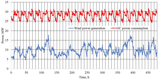
E3S Web of Conferences 209, 02020 (2020) https://doi.org/10.1051/e3sconf/202020902020
ENERGY-21
2 The Problem Statement
2.1 GC Power System
In this research, we considered two large GC: the power
system of Russky Island and the power system of Popov
Island. Both islands are located in Peter the Great Gulf in
the East Sea (Fig. 1). High wind speed makes it possible
to create wind power plants up to 16 MW on Russky
Island and up to 20 MW on Popov Island [16].
Russky Island belongs to the territorial composition
of Vladivostok. It is located about two kilometers from
the coast in Peter the Great Gulf, which is part of the Sea
of Japan (the smallest distance between the continental
part and the island is 800 meters). Russky Island is
separated from the Muravyov-Amursky Peninsula by the
East Bosphorus. From the west, the island is washed by
the waters of the Amur Gulf, and from the east and south
Fig. 1. Russky and Popova Islands.
side by the waters of the Ussuri Gulf. In the southwest,
the island is separated from the other Popov island by the
Stark Strait.
The island is 97.6 km2, its length is about 18 km, and
its width is about 13 km. The population of the island is
approximately 25,000 inhabitants.
Popova Island (named after Admiral A.A. Popova) is
located in Peter the Great Gulf of the Sea of Japan, 20
km from Vladivostok and 0.5 km southwest of Russky
Island. About 3,000 people live on the island, mainly in
the two villages of Stark and Popova.
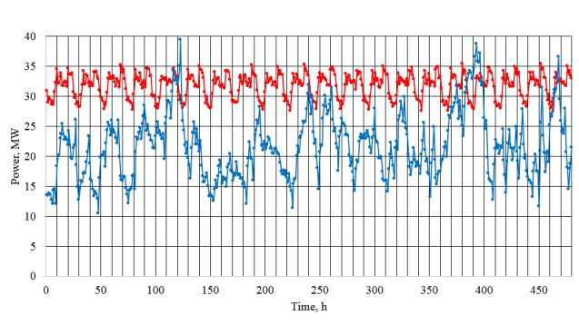
Fig. 2 and Fig 3. show curves of own consumption of Fig. 2. Consumption and generation of Russky GC.
Russky GC and Popova GC and possible wind power
generation of GCs according to the estimates of [16]. Fig
4. shows the results of adding these curves. The
demonstrated fragment of data corresponds to twenty
days from 01.06.2017.
From the charts above it is possible to notice the
following:
• the forms of the electricity generation curves are very
close since both islands are located very close, and their
wind speeds are also close;
• the load curves concerning to generation are radically
different; the Russky GC always has a deficit, the Fig. 3. Consumption and generation of Popova GC.
Popova GC still has a surplus;
• in case of consideration of two consumers together, we
have the third type of load / generation pattern – in
general, the GC system has a deficit, but sometimes
there is a surplus.
Thus, different management strategies may be
required depending on the characteristics of GC or GC
hub.
2.2 Optimal Control
The task of optimal control is to create a control system Fig. 4. Aggregated consumption and generation of both GC.
(subject) that implements a sequence of actions on a
controlled object in the environment to achieve the best The state of the controlled object is characterized by
possible quality specified by one or more criteria (Fig. a set of parameters that can change over time:
5); the controlled object is a specific part of the world
around which the control subject can purposefully S(t) = {s1(t), s2(t), ..., sn(t)}. (1)
influence [17]. Control always occurs during a certain
Thus, there is a vector of functions. Each function shows
period of time, while the controlled object passes from
the parameter changing over time. These functions in the
one state to another.
2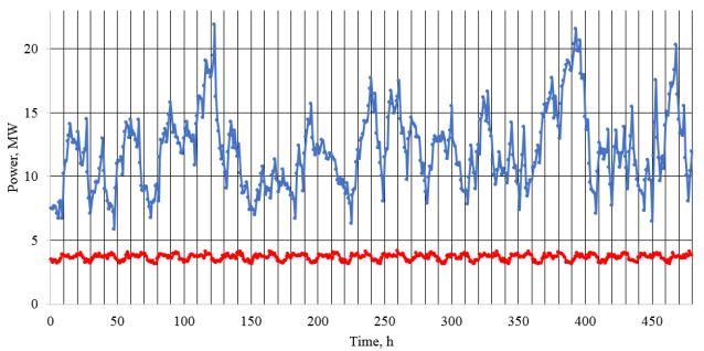
E3S Web of Conferences 209, 02020 (2020) https://doi.org/10.1051/e3sconf/202020902020
ENERGY-21
explicit form are unknown. In addition, there is a control cannot usually be obtained, especially integral of this
system that provides control. function. But it is possible to calculate the function
algorithmically. In the case of GC control, this function
is piecewise continuous, since the time step is 1 hour.
The task (3) can be written without an integral, in the
form of a sum, and the function f(t, S(t), A(t)) is nothing
more than the difference between the revenues from the
sale of electricity of a GC and the costs of its purchase,
generation, and power storage in all hours into the time
period. However, even in this case, the analytical
Fig. 5. Interaction between a subject and an object. expression for f(t, S(t), A(t)) is difficult to write, since the
price of electricity is a piecewise constant function, the
The control can also be defined as a vector of exchange of electricity with a neighboring GC supply
functions: depends on its state and controlling them. Thus, the
calculation of the value of f(t, S(t), A(t)) should be
A(t) = {a1(t), a2(t), ..., am(t)}. (2) performed algorithmically:
T
The notations S from “state” and A from “action” are Aopt (t ) arg min revenue t , S t , A t (4)
used. A ( t ) A pos t t0
The optimal control problem, in general, can be
written as follows:
tT
Aopt (t ) arg min f t , S t , A t dt (3)
A ( t ) A pos t
0
• Aopt(t) is the required optimal control; it defines values
of the control parameters at each time moment (in the
considered task, when and how much GC must sell or
buy, charge or discharge);
• Apos is the area of permissible values of control
parameters;
• f(t, S(t), A(t)) is a continuous-time cost function, in the
considered task, it gets GC’s total electricity costs: Fig. 6. Sample of daily state-action curves of Russky GC.
purchases from the own generation + purchases from the
other GC and an external power system – sale to other 3 The Research Method
GC and the external power system.
• t0 and tT are the period of time considered.
3.1 Heuristic-Rule-based control
2.3 GC Optimal Control task All possible control actions could be described by
dividing them into four groups. The following
For GC, the state parameters can be defined as follows: designation is used:
• own consumption, MWh (s1); • power_wind – GC wind power plant generation at the
• wind power plants generation, MWh (s2); considered hour;
• charge level of power storage, MWh (s3). • power_gc – GC consumption at the considered hour;
Control parameters can be defined as follows: • dif – the difference between the GC generation and
• the amount of electricity that is currently exchanged by consumption at the considered hour;
the GC with an external power system (purchase or sale), • storage – the amount of energy that needs to be
MWh (a1); charged (> 0) or discharged (E3S Web of Conferences 209, 02020 (2020) https://doi.org/10.1051/e3sconf/202020902020
ENERGY-21
• sale_buy – the amount of energy that is sold (> 0) or has four balance factors: buy_unload, sale_unload,
purchased ( the procedure for their verification and compliance, that
consumption). is, rule priorities. Decision making begins with checking
1.1. dif = power_wind - power_gc; of the highest priority rule. If its condition is satisfied,
1.2. storage = min(max_storage – now_storage, then the corresponding action of this rule is
max_storage_h, dif); implemented. Otherwise, the next priority rule is
1.3. storage = storage * sale_storage; checked, and so on until the end of the rule list. The
1.4. now_storage = now_storage + storage; conditions are designed in such a way that when you go
1.5. sale_buy = dif – storage. through the list of rules, you will surely find one whose
2. Charge_Buy: condition will be satisfied. As a result, to build a
2.1. dif = power_wind - power_gc; controller, it is necessary to determine the order of the
2.2. storage = min(max_storage – now_storage, rules by setting priorities (pri) and the tuned parameters
max_storage_hour); specified above:
2.3. storage = storage * buy_storage;
2.4. now_storage = now_storage + storage; Solution = [pr1, …, pr12, buy_unload, sale_unload,
2.5 sale_buy = dif – storage. buy_storage, sale_storage, time1, … , time4]
3. Discharge_Sell:
3.1. dif = power_wind - power_gc; 3.2 Swarm Intelligence
3.2. storage = now_storage;
3.3. storage = storage * sale_unload; It is not always possible to determine the Swarm
3.4. now_storage = now_storage – storage; Intelligence algorithm that is most suitable for a solved
3.5. sale_buy = dif + storage. task [15]. Therefore, the use of only one algorithm can
4. Discharge_Buy (it’s possible if generation < give a solution whose effectiveness is not satisfactory for
consumption): the optimization criterion. In this case, the researcher
4.1. dif = power_wind - power_gc; cannot determine the effectiveness without using other
4.2. storage = min(–dif, now_storage); algorithms for comparison. Therefore, three Swarm
4.3. storage = storage * buy_unload; Intelligence algorithms were applied: the Particle Swarm
4.4. now_storage = now_storage – storage; Optimization (PSO) algorithm, the Firefly Optimization
4.5. sale_buy = storage – dif. (FFO) algorithm, and the Bees algorithm (BA) (not
The choice of actions should depend on the state of Artificial Bee Colony Optimization). Descriptions of the
the GC, but it is enough to get answers to two questions. algorithms precisely in the form in which they are
The first is connected with determining whether the GC applied in this research are given in.
is in a state of excess or deficiency of energy? The
second is also related to the fact that the price of
3.2.1 Particle Swarm Optimization
electricity changes throughout the day. Although various
billing schemes are possible, a two-zone tariff is The Particle Swarm Optimization algorithm was first
considered in this research, the daily tax is from 7 a.m. to proposed by J. Kennedy and R. Eberhart in 1995 [18].
11 p.m., and at other hours it is a night tax, cheaper one. Then it was improved by Kennedy, Eberhart, and Shi
Thus, it’s needed to get answers to the questions: [19]. PSO is based on a bird flocks’ behavior. A flock
1) Excluding accumulation, does the generation of acts coordinated according to a number of simple rules.
the GC wind power plant more than the GC consumption Every bird (called particle) coordinates own movements
(diff> 0)? with the movements of whole flocks. In the PSO
2) Is there a special time period now? algorithm, every particle is denoted by a position vector,
The GC control takes into account the possibility of a velocity vector, and a value of the criterion. The
using two intervals as special periods (from time1 to vectors of position and velocity of all particles are
time2 and from time3 to time4), the values of the updated according to a number of rules taking into
boundaries of the time intervals are parameters adjusted account the best position of a particle, and the best
during the optimization process. position of the whole swarm. Also, the algorithm uses
As a result, we have four possible cases at each hour: inertia weights of the particles, velocities restriction and
• (diff < 0) AND NOT (special_time_period); the stochastic deviations.
• (diff > 0) AND NOT (special_time_period); According to the scheme of the swarm algorithms
• (diff < 0) AND (special_time_period); description [15], the PSO algorithm may be represented
• (diff > 0) AND (special_time_period). by a tuple {S, M, A, P, I, O}.
When creating a GC control based on rules, we get 1. A set of particles (particles) S = {s1, s2,…,s|S| }, |S|
12 rules of the form IF , THEN is number of particles. At j-th iteration i-th particle is
The number of rules is 12 since the second and third characterized by the state sij = {Xij,Vij, Xbestij}, where Xij =
actions can be performed under any of the four {x1ij, x2ij,…, xlij} is the variable parameter vector (particle
conditions, and the first and fourth under two conditions position), Vij = {v1ij, v2ij,…, vlij} is the velocity vector,
(2 * 4 + 2 * 2 = 12). In addition, the GC control model
4E3S Web of Conferences 209, 02020 (2020) https://doi.org/10.1051/e3sconf/202020902020
ENERGY-21
Xbestij = {b1ij, b2ij,…, blij} are the best (by value) fitness- the more bees go to it. However, the bees can randomly
functions of the particle position among all the positions deviate from the chosen direction. After the return of all
it took during the algorithm operation from the 1 st to the the bees in the hive, information exchange and sending
j-th iterations, l is the number of variable parameters. of bees again.
2. Means of indirect exchange is vector M = Xbestj is According to the description scheme of swarm
the best value of the variable parameters vector derived algorithms, the BA algorithm may be represented by a
among all particles from the 1st to the j-th iterations of tuple {S, M, A, P, I, O}.
the algorithm. 1. A set of particles (bees) S = {s1, s2, …, s|S|}. At the
3. Algorithm A describes the steps of the PSO j-th iteration the i-th particle is characterized by the state
algorithm. sij = {Xij}, where Xij= {x1ij, x2ij, …, xlij,}is the variable
3.1. Generation of initial population (iteration parameters vector (the particle position), l is the
number j = 1): dimensionality of the solution search space.
Xi1 ← random(0,1), i = 1, …, |S|, 2. Means of indirect exchange M is a list of the best
Vi1 ← random(0, vmax), i = 1,…|S|, and perspective positions found in the j-th iteration, M =
Xbesti1 ← Xij, i = 1, …|S|, {Nijb, Nkjg}, i = 1, ..., nb, k = 1, ..., ng.
where random(0, 1) is the vector of random numbers 3. Algorithm A describes the steps of the BA
with dimensionality l (dimensionality of solution search algorithm.
space) uniformly distributed from 0 to 1. 3.1. Generation of initial population (j=1) is fulfilled
3.2. Calculation of fitness- functions. The criterion only for a subset of particles termed scouts:
calculation takes place in the mathematical model of the Xi1 ← random(0,1), i = 1, …, ns,
problem where Xij vectors are entered from algorithms where ns is the number of scout particles. Other
and the results are returned to the algorithm through the particles are considered as inactive this time (only at the
interface {I, O}. first iteration).
Xbestij ← Xij | f(Xbestij)1 , i = 1, …, |S|. the lists of the best and perspective positions M = (Nijb,
Xij+1 ← 0| Xij+1E3S Web of Conferences 209, 02020 (2020) https://doi.org/10.1051/e3sconf/202020902020
ENERGY-21
the total number of the swarm particles (|S| = ns + nbсb + Where random ∈ [0, 1], and G(X) is used in this case
ngсg). The selection of the algorithm parameters heavily as the predicate showing if X belongs the area of
affects the quality of derived solutions, so in order to admissible solutions.
increase the algorithm efficiency it is necessary to adapt The function v(Xij, Xkj) defines the attractiveness of k
parameters. particle for i particle with j algorithm iteration:
v(Xij, Xkj) ← β·(1 + γ·r(Xij, Xkj))-1
where r(Xij, Xkj) is Cartesian distance between
3.2.3 Firefly Optimization
particles.
Firefly Optimization was proposed by Xin-She Yang in 3.4. If at the j-th iteration a stop-condition is
2010 [21]. This algorithm as all Swarm Intelligence satisfied, then the value Xbesti is transmitted to output O,
algorithms is based on the particles (fireflies) movement or the transition to iteration 3.2 takes place.
in the search searching space. Let’s consider the 4. Vector P = {α, β, γ} are coefficients of the
objective function minimum problem of the following algorithm. Coefficient α determines the influence degree
type f(X), where X is a vector of varied parameters which of stochastic algorithm nature. Coefficient β sets the
can get the values from some D area. Each particle is degree of attraction between particles with zero distance
specified by the value of X parameter and value of an between them i.e. defines the particle’s mutual influence.
optimized function f(X). Thus, the particle is a feasible Coefficient γ controls the dependence of attraction on the
solution of the considered optimization problem. distance between particles.
As the algorithm is based on watching for fly’s
behavior, each particle is considered to see the “light” 3.3 Application the Swarm Intelligence
from their neighbors, but the brightness of the “light” Algorithm for GC optimal control
depends on the distance between particles. For the
process of solution finding to be converged to the For applying SI algorithms, it is necessary to determine
optimum, each particle in its movement takes into the mapping of the particle coordinate (X) in the search
account only those neighbors having a better value of space solution to the solutions of the solved task. In this
f(X) criterion. But for the algorithm not to degenerate case, the solution is the control actions A(t), as shown in
into greedy heuristics, it is necessary to have particles’ expression (1). Each element of the vector X is bounded
stochastic movement. from 0 to 1 [15]. The priorities are real numbers from 0.0
According to the description scheme of swarm to 1.0, so pri = xi, i = 1, ..., 12. The parameters
algorithms, the FFO algorithm may be represented by a buy_unload, sale_unload, buy_storage, sale_storage
tuple {S, M, A, P, I, O}. also take values from 0.0 to 1.0, so they are mapped in
1. Set of particles (fire-flies). S = {s1, s2, …, s|S|}, |S| the same way. To set values of time1, ..., time4, we use
is a number of particles. At iteration j the ith particle is rounded down values of 24x17, …, 24x20.
specified by the state sij = {Xij}, where Xij = {x1ij, x2ij, …, The FFO algorithm requires comparing each particle
xlij} is a vector of the varied parameters (particle’s to each other, so the number of operations quadratically
position), l is a number of the varied parameters. depends on the number of particles. The PSO and BA
2. Means of indirect exchange is vector M is have a linear relationship. We reduce the number of FFO
particles’ brightness. particles to equalize the calculation time. At the same
M = {f(X1j), f(X2j), f(X|s|j)} time, we increase the number of iterations of the FFO
Brightness is determined by the optimality criterion. algorithm to equalize the number of calculations of the
This vector ensures the indirect experience exchange objective function. As a result, the number of particles is
among particles. reduced four times, and the number of iterations is
3. Algorithm A describes the steps of the ACO increased four times compared to the PSO algorithm and
algorithm. the BA. The parameters of the SI algorithms are given in
3.1. Generation of initial population (iteration Table 1.
number j = 1):
Xi1 ← random(G(X)), i = 1, …, |S|, Table 1. Parameters of the SI algorithms
where random(G(X)) is a vector of equally
distributed random variables meeting the restrictions of Alg. Particles Iteration Heuristic coefficients
searching space.
3.2. Calculation of fitness-functions. The criterion α1 = 1.5 α2 = 1.5,
calculation takes place in the mathematical model of the PSO 200 500
ω = 0.7, β = 0.5
problem where Xij vectors are entered from algorithms ns = 60, nb = 6, ng = 1,
and the results are returned to the algorithm through the BA 200 500 сb = 20, cg = 20,
interface {I, O}. rad = 0.01, rx = 0.05
mij ← f(Xij), i = 1, …, |S|
Xjbest ← Xij | f(Xij) ≤ f(Xjbest) FFO 50 2000 α = 0.05, β = 1, γ = 0.5
3.3 Particles’ movement:
Xij+1 ← Xij + v(Xij, Xkj) · (Xij – Xkj) + α·random(0, 1) |
mkj ≤ mij , i, k = 1, …, |S|, i ≠ k,
if G(Xij+1) = 0, Xij+1 ← Xij , i = 1, …, |S|,
6E3S Web of Conferences 209, 02020 (2020) https://doi.org/10.1051/e3sconf/202020902020
ENERGY-21
4 Results and Discussion For the GC of Russky Island, there is a situation of
electricity shortage, so control does not make a large
contribution. For the Popova Island GC, on the contrary,
4.1 Computational Experiment there is an excess of electricity; therefore, it is necessary
Computational experiments were carried out while to determine the best moments for the sale of electricity
considering the GC of Russky and Popov Islands (GCR, and the balance between sale and accumulation.
GCP, respectively). Table 2 shows the prices used in the The most interesting situation is when a joint system
simulation. of two GCs is controlled together. First, in this case, the
profile is more complicated (Fig. 4), since there are
Table 2. Prices used in the simulation moments of both excess and shortage of electricity.
Secondly, the power storage capacity is two times higher
Price, Price, due to the combination of storages of both GC in a single
Power flow
rubel / MWh $ / MWh power system. Thirdly, the combined GC has a higher
Wind generation 500 6,67 generation and consumption, since, it is evident that all
Power storage quantitative indicators will be more top.
100 1,33 The results of all applied SI algorithms are very
discharging
Sale (daily rate) 3200 42,7 close, even without adjusting the heuristic parameters. It
can be explained by the relatively low complexity of the
Sale (daily rate) 1400 18,67 task from the point of view of optimization theory since
Buy (daily rate) 2700 36,00
there are not many control options.
Buy (daily rate) 900 12,00
To evaluate the effectiveness of the rule-based
control model built by the Swarm algorithms, we
compared them with a base constructed manually by an
expert. The main advantage of using SI is an automatic
adaptation to the profiles of production and consumption
of each GC. Therefore, the expert rules were constructed
one time for the general case.
Obviously, in the problem under consideration,
control is impossible without power storage. Because
without it, GC has to sell electricity at times of excess
and buy at times of shortage, and there are no other
options. Therefore, control efficiency is limited by the
capacity of the power storage. Due to the limitation of
capacity and the use of tariff simulation with only two Fig. 7. Algorithms’ results. The histogram shows the monthly
rates (day, night), the reduction in energy consumption profit ($) of power storage usage with the different algorithms
or the increase in income (this is the same thing) is not of optimize control rule-based model. Left 4 bars shows results
very large. Thus, for results clarification, we did not for GCR, central 4 bars – for GCP, right 4 bars – for GCR+P.
compare the absolute values of the cost of electricity
according to criterion (4), but the benefits that control Table 3. Algorithms’ results
gives regarding the situation without power storage.
In section 2.1, three cases are considered: the control Cost, Monthly Profit,
Case Algorithm
of a GC of Russky Island, GC of Popova Island, and an thousands $ thousands $
integrated system of both GCs. For each situation and GCR No 580.3 -
each algorithm, modeling was performed on data for two GCR Expert 579.8 0.241
summer months (Fig. 2-4). GCR PSO 579.4 0.43
GCR BA 579.5 0.43
GCR FFO 579.5 0.43
4.2 Simulation results
GCP No -41.6 -
Table 3 shows the results. Each SI algorithm was GCP Expert -41.5 0
launched 20 times, and in 17-18 launches out of 20 gave GCP PSO -42.8 0.6
the same result. This result is used as a summary. The GCP BA -42,8 0.59
results without the use of power storage are shown in GCP FFO -42,8 0.59
rows with the label "No" in the "Algorithm" column, and GCR+P No 452,0 -
the results of control using the expert rules are labeled as GCR+P Expert 450,4 0.57
"Expert". Also, Fig. 7 visualizes the benefits of using the GCR+P PSO 447,3 2.33
rule-based model optimized by the SI. GCR+P BA 447,3 2.33
It can be seen that the difference varies greatly GCR+P FFO 447,3 2.33
depending on the profile of production and consumption.
7E3S Web of Conferences 209, 02020 (2020) https://doi.org/10.1051/e3sconf/202020902020
ENERGY-21
5 Conclusion Using Internet of Things in Smart Grid Demand
Response Management. IEEE Transactions on
In this research, we have applied Swarm Intelligence Industry Applications, 53.6, pp. 5155-5163 (2017)
algorithms to optimize the heuristic-rule-based control 9. S.R. Etesami, W. Saad, N.B. Mandayam, H.V. Poor.
model (optimize priorities of rules and numerical values Stochastic Games for the Smart Grid Energy
of the model coefficients) for optimal control of Management with Prospect Prosumers. IEEE
generating consumers with wind power plants. The Transactions on Automatic Control, 63.8, pp. 2327-
computer simulation showed that SI allowed to increase 2342 (2018)
the profit of power storage usage 1.8–4.1 times
compared with the rules build by experts. The simulation 10. G. El Rahi, et. al. Managing Price Uncertainty in
results confirmed that it is appropriate to apply the SI Prosumer-Centric Energy Trading: A Prospect-
algorithms to increase accuracy of heuristic-rule-based Theoretic Stackelberg Game Approach.
model, and perform adaptation to a given generating Transactions on Smart Grid, 10.1, pp. 702-713
consumer. (2019)
The proposed control model allows to get the robust 11. N. Liu, X. Yu, C. Wang, J. Wang. Energy Sharing
control in a particular situation, which can be easily Management for Microgrids with PV Prosumers: A
transferred to other climatic conditions and GC features. Stackelberg Game Approach. IEEE Transactions on
For future work, we plan: firstly, to complicate a GC Industrial Informatics, 13.3, pp. 1088-1098 (2017)
model and a model of GCs interaction; secondly, to 12. Y. del Valle, et al. Particle Swarm Optimization:
apply the Q-learning method for the optimal control of Basic Concepts, Variants and Applications in Power
GC; thirdly, make comparisons with existing methods Systems. IEEE Transactions on Evolutionary
using larger dataset. Computation, 12.2, pp. 171-195 (2008)
13. V.Z. Manusov, P.V. Matrenin, L.S. Atabaeva.
This work is supported the Novosibirsk State Technical Firefly Algorithm to Optimal Distribution of
University Development Program through the Project C20-20. Reactive Power Compensation Units. International
Journal of Electrical and Computer Engineering,
8.3, pp. 1758-1765 (2018)
References
14. V.Z. Manusov, et al Optimization of Power
1. C.W. Gellings. The Smart Grid: enabling energy Distribution Networks in Megacities. IOP
efficiency and demand response. (Lilburn, CA: Conference Series: Earth and Environmental
Fairmont Press, 2009). Science. International Conference on Sustainable
2. V.Z. Manusov, N. Khasanzoda, P.V. Matrenin. Cities, 72, id 012019 (2017)
Application of artificial intelligence methods to 15. V.Z. Manusov, P.V. Matrenin, S.E. Kokin. Swarm
energy management in Smart Grids (Novosibirsk, Intelligence Algorithms for The Problem of The
2019) [In Russian] Optimal Placement and Operation Control of
3. X. Fang, S. Misra, G. Xue, D. Yang. Managing Reactive Power Sources into Power Grids.
smart grid information in the cloud: Opportunities International Journal of Design & Nature and
model and applications. IEEE Netw., 26.4, 32-38 Ecodynamics, 12.1, pp.101-112 (2017)
(2012). 16. N. Khasanzoda. Optimization of power consumption
4. R. Zafar, et. al. Prosumer based energy management modes in intelligent networks with a two-way flow of
and sharing in smart grid. Renewable and energy using artificial intelligence methods
Sustainable Energy Reviews, 82.1, pp. 1675-1684 (Novosibisk, 2019) [In Russian]
(2018) 17. L.A. Rastrigin, Modern principles of management of
5. A.G. Azar, et. al. A Non-Cooperative Framework complex objects (Moskov, 1980) [In Russian]
for Coordinating a Neighborhood of Distributed 18. J. Kennedy, R. Eberhart. Particle swarm
Prosumers. IEEE Transactions on Industrial optimization. IEEE International Conference on
Informatics, 15.5, pp. 2523-2534 (2019) Neural Networks, Perth, WA, Australia. pp. 1942–
6. L. Ma, N. Liu, J. Zhang, L. Wang. Real-Time 1948 (1995)
Rolling Horizon Energy Management for the 19. R.C. Eberhart, Y. Shi. Particle swarm optimization:
Energy-Hub-Coordinated Prosumer Community developments, applications and resources. Congress
From a Cooperative Perspective. IEEE Transactions on Evolutionary Computation; Seoul, South Korea.
on Power Systems, 34.2, pp. 1227-1242 (2019) pp. 81-86 (2001)
7. A.C. Luna, N.L. Diaz, M. Graells, J.C. Vasquez, 20. D.T. Pham, et. al. The bees algorithm – a novel tool
J.M. Guerrero. Cooperative energy management for for complex optimisation problems (Cardiff, UK,
a cluster of households prosumers. IEEE 2005)
Transactions on Consumer Electronics, 62.3, pp. 21. X. Yang. Firefly algorithm, Stochastic Test Function
235-242 (2016) and Design Optimization. International Journal of
8. H. Mortaji, S. Siew, M. Moghavvemi, H. Almurib. Bio-Inspired Computation. 2.2, pp. 78-84 (2010)
Load Shedding and Smart-Direct Load Control
8You can also read