Model-Free Control as a Service in the Industrial Internet of Things: Packet loss and latency issues via preliminary experiments - arXiv
←
→
Page content transcription
If your browser does not render page correctly, please read the page content below
Model-Free Control as a Service
                                                                               in the Industrial Internet of Things:
                                                                                   Packet loss and latency issues
                                                                                    via preliminary experiments
                                                                                 Cédric Join1,3 , Michel Fliess2,3 , Frédéric Chaxel1

                                                                                                              Abstract
                                                   Model-Free Control (MFC), which is easy to implement both from software and hardware viewpoints, permits the intro-
                                               duction of a high level control synthesis for the Industrial Internet of Things (IIoT) and the Industry 4.0. The choice of the
                                               User Diagram Protocol (UDP) as the Internet Protocol permits to neglect the latency. In spite of most severe packet losses,
arXiv:2004.12156v2 [eess.SY] 4 Jun 2020

                                               convincing computer simulations and laboratory experiments show that MFC exhibits a good Quality of Service (QoS) and
                                               behaves better than a classic PI regulator.
                                                                                                         Index Terms
                                                     Control engineering, model-free control, intelligent controllers, industrial internet of things, industry 4.0, cyber-physical
                                                 systems, cloud computing, latency, packet loss, congestion, UDP protocol, half quadrotor, joystick.

                                                                                                        I. I NTRODUCTION
                                              The conceptual meanings of the buzzwords Industrial Internet of Things (IIoT) (see, e.g., [8], [25]), industry 4.0 (see,
                                          e.g., [17], [41]), cyber-physical systems (see, e.g., [34]) do overlap to some extent (see, e.g, [17], [21]). Control engineering
                                          (see, e.g., [4]) plays there a key rôle (see, e.g., [33], [51]) via networks that are often related to cloud computing (see, e.g.,
                                          [32], [35]).
                                              Among the numerous existing control strategies, model predictive control (see, e.g., [9]) seems today the most popular
                                          one, at least in the academic literature (see, e.g., [1], [3], [10], [18], [27], [28], [36], [44], [47], [48]). This communication
                                          advocates Model-Free Control (MFC) in the sense of [13], and the corresponding “intelligent” controllers. This setting,
                                          which is easy to implement both from software [13] and hardware [22] viewpoints, will hopefully lead in some near future
                                          to Model-Free Control as a Service (MFCaaS). It has been already most successfully applied in many concrete situations
                                          (see the references in [13] and [5] for a quite complete listing until the beginning of 2018). Some have been patented. The
                                          recent contributions of MFC to the dynamic adaptation of computing resource allocations under time-varying workload in
                                          cloud computing [6] and to the air-conditioning of data centers [14] should be emphasized here.
                                              The choice of an appropriate Internet Protocol (IP) stack is of utmost importance in this networking context (see, e.g.,
                                          [30]). It is obvious that packet loss and latency, which are unavoidable, might significantly degrade the performances of any
                                          control law. There are two main protocols of transport layer, the Transmission Control Procol (TCP) and the User Datagram
                                          Procol (UDP) (see, e.g., [29], [45], [46] for some details). TCP is more reliable but may exhibit often fatal latency and
                                          jitter. This is why we select here UDP, which is faster:
                                             • It permits to neglect the delay if the transmission distance is not “too” large (see Section V).
                                             • Only packet loss, which might be most severe, is taken into account (compare, e.g., with [37]).
                                             • Packets that arrive late are discarded.
                                             • Congestion may therefore be somehow ignored.
                                          This communication, which completes a recent technical report [24], is organized as follows. Basic facts about MFC are
                                          summarized in Section II. Section III is devoted to computer simulations. After the introduction of two types of packet
                                          loss in Section III-A, a single tank is analyzed in Section III-B: the computer simulations for MFC indicate in spite of
                                          serious packet losses a fine Quality of Service (QoS), which is much better than with a classic PI. Those ascertainments
                                          are confirmed in Section IV via laboratory experiments with the Quanser AERO, i.e., a half quadrotor. In Section IV-C a
                                          joystick is added. See Section V for some suggestions on prospective studies.
                                            1 CRAN    (CNRS, UMR 7039)), Université de Lorraine, BP 239, 54506 Vandœuvre-lès-Nancy, France.
                                          {Cedric.Join, Frederic.Chaxel}@
                                          univ-lorraine.fr
                                            2 LIX   (CNRS, UMR 7161), École polytechnique, 91128 Palaiseau, France. Michel.Fliess@polytechnique.edu
                                            3 AL.I.E.N. (ALgèbre pour Identification & Estimation Numériques), 7 rue Maurice Barrès, 54330 Vézelise, France.
                                          {cedric.join, michel.fliess}@alien-sas.com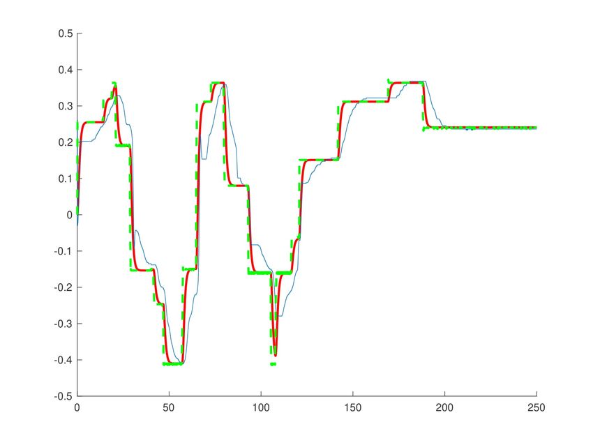
II. M ODEL - FREE CONTROL AND INTELLIGENT CONTROLLERS1
A. The ultra-local model and intelligent controllers
  For the sake of notational simplicity, let us restrict ourselves to single-input single-output (SISO) systems. The unknown
global description of the plant is replaced by the following first-order ultra-local model:
                                                          ẏ = F + αu                                                         (1)
where
 1) the control and output variables are respectively u and y,
 2) α ∈ R is chosen by the practitioner such that the three terms in Equation (1) αu are of the same magnitude.
The following comments are useful:
 • F is data driven: it is given by the past values of u and y.
 • F includes not only the unknown structure of the system but also any disturbance.

  Close the loop with the intelligent proportional controller, or iP,
                                                           Fest − ẏ ∗ + KP e
                                                    u=−                                                                       (2)
                                                                    α
where
     ∗
 • y is the reference trajectory,
              ?
 • e = y − y is the tracking error,
 • Fest is an estimated value of F ,
 • KP ∈ R is a gain.
Equations (1) and (2) yield
                                                     ė + KP e = F − Fest                                                     (3)
If the estimation Fest is “good”: F − Fest is “small”, i.e., F − Fest ' 0, then limt→+∞ e(t) ' 0 if KP > 0. It implies that
the tuning of KP is quite straightforward. This is a major benefit when compared to the tuning of “classic” PIDs (see, e.g.,
[4], [39]).
   Remark 2.1: See [13], [23] for other types of ultra-local models, where the derivation order of y in Equation (1) should
be greater than 1, and for the corresponding intelligent controllers. The extension to MIMO systems is straightforward [31].
B. Estimation of F
   Mathematical analysis (see, e.g., [7]) tells us that under a very weak integrability assumption, any function, for instance
F in Equation (1), is “well” approximated by a piecewise constant function. The estimation techniques below are borrowed
from [16], [43].
   1) First approach: Rewrite then Equation (1) in the operational domain (see, e.g., [50]):
                                                           Φ
                                                    sY =     + αU + y(0)                                                      (4)
                                                           s
                                                                                                             d
where Φ is a constant. We get rid of the initial condition y(0) by multiplying both sides on the left by     ds :
                                                         dY       Φ      dU
                                                   Y +s      =− 2 +α                                                          (5)
                                                         ds       s      ds
Noise attenuation is achieved by multiplying both sides on the left by s−2 . It yields in the time domain the real-time estimate,
                                    d
thanks to the equivalence between ds    and the multiplication by −t,
                                                 Z t
                                               6
                                 Fest (t) = − 3        [(τ − 2σ)y(σ) + ασ(τ − σ)u(σ)] dσ
                                              τ t−τ
where τ > 0 might be quite small. This integral, which is a low pass filter, may of course be replaced in practice by a
classic digital linear filter.
   2) Second approach: Close the loop with the iP (2). It yields:
                                                    Z t
                                                  1
                                       Fest (t) =          (ẏ ? − αu − KP e) dσ
                                                  τ t−τ
  1 See   [13] for more details.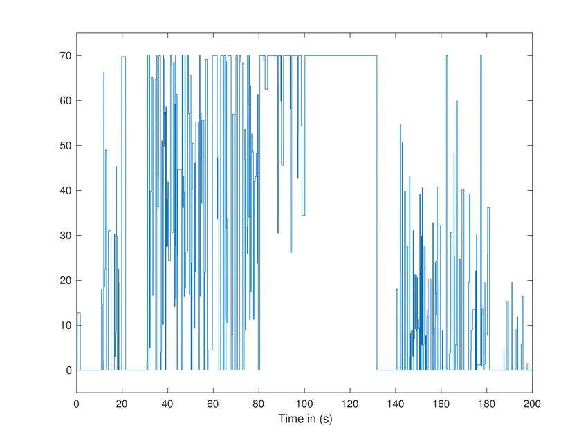
III. C OMPUTER EXPERIMENTS
A. Generalities
We use an intelligent proportional controller, i.e., Formula (2), where F and u are obtained thanks to a computer server
which is connected to the plant via UDP. Two types of packet loss are considered :
• Fault 1 – Some measurements of the sensor y do not reach the server. The estimation of F and u is frozen.
• Fault 2 – The calculations of the server do not reach the plant. The control variable u is thus frozen, but not the
estimation of F .
B. A single tank
1) Model-free control: The following mathematical model is only useful for computer simulations:2
√
u − 0.2700K y
ẏ = 0 < y < 60, 0 < u < 70 (6)
5
The outlet valve opening K, 0 < K < 100, should be viewed as an unknown perturbation. The output is corrupted by an
additive band-limited white noise of power 0.025 (see, e.g.,[42]). The sampling time is 100ms. The simulations duration is
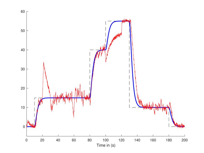
equal to 200s. The reference trajectory y ∗ , which is piecewise constant, explores all the possibilities: y ∗ (t) = 0 if 0 ≤ t < 10s,
y ∗ (t) = 15 if t < 10 ≤ t < 80s, y ∗ (t) = 40 if 80 ≤ t < 100s, y ∗ (t) = 55 if 100 ≤ t < 130s, y ∗ (t) = 10 if 130 ≤ t < 180s,
y ∗ (t) = 0 if 180 ≤ t < 200s. Set K = 10 if 0 ≤ t < 30, K = 50 if 30 ≤ t < 120, K = 20 if 120 ≤ t < 200. Set in Formula
(2) α = 0.1, KP = 0.5. In order to assess the effects of the packet loss 5 scenarios are considered:
• Scenario 1 – Tracking of the reference trajectory and no packet loss.
• Scenario 2 – Fault 1 (resp. 2) occurs if 140 ≤ t < 150 (resp. 50 ≤ t < 60).
• Scenarios 3, 4 & 5 – There is 30% (resp. 50%, 70%) of packet loss. Both types are evenly distributed
Figures 1-3 display strong performances in spite of a big packet loss and significant variations of the parameter K. The poor
tracking of the setpoint when 100 < t < 120 is due to the saturation of control variable u and not to the packet loss.
2) A comparison with a PI controller: Consider a classic PI controller (see, e.g., [4], [39]) where e is the tracking error,
kp , ki ∈ R are the gains: Z
u = kp e + ki e (7)
Set for the tank K = 30 and for Formula (7) kp = 29.69, ki = 2.27009.3 The results in Figure 1-(c) are rather good without
any packet loss, although u (see Figure 1-(d)) is quite sensitive to the corrupting noise. When the packet loss become
important Figure 5 shows a poor tracking. The malfunction depicted in Figure 4 is due to the usual anti-windup, which is
related to the integral term in Equation (7) (see, e.g., [4], [39]).
Remark 3.1: In another situation, where a delay cannot be neglected, it has been shown [20] that our iP behaves better
than a classic PI.
IV. E XPERIMENTS WITH THE Q UANSER AERO
A. Quick presentation
The Quanser AERO4 is a half-quadrotor, which “is a fully integrated dual-motor lab experiment, designed for advanced
control research and aerospace applications.” Two motors driving the propellers, which might turn clockwise or not, are
controlling the angular position y (rad) of the arms. Write vi , i = 1, 2, the supply voltage of motor i, where −24v ≤ vi ≤ 24v
(volt).
B. Some experiments
The single control variable u in Equation (1) is defined by
• if u > 0, then v1 = 10 + u, v2 = −10 − u
• if u < 0, then v1 = −10 + u, v2 = 10 − u.
In Equations (1)-(2) moreover, α = 5, KP = −10. Everything is programed in C# and stored in the server. It computes
u and Fest , every 10ms, according to the process interface instructions. Consider again the types of packet loss of Section
III-A. The duration of the experiments is equal to 250s. Three scenarios are examined:
2 See the real-time Matlab example:
https://fr.mathworks.com/help/sldrt/ug/
water-tank-model-with-dashboard.html?s tid=srchtitle
3 Those numerical values are obtained via the Broı̈da method which is very popular in France (see, e.g., [39]).
4 Seethe link
https://www.quanser.com/products/quanser-aero/
where a detailed picture is available.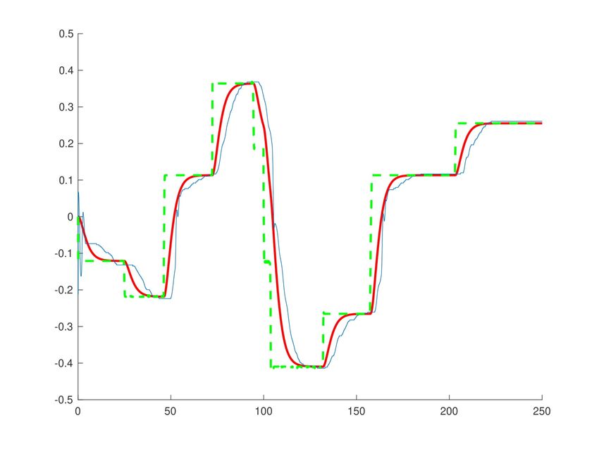
(a) MFC: output variable (red), setpoint         (b) MFC: control variable    (c) PI: output variable (red), setpoint
               (black) and reference trajectory (blue)                                       (black) and reference trajectory (blue)

                                                              (d) PI: control variable
                                                         Fig. 1: Scénario 1: MFC & PI

           (a) PI: output variable (red), setpoint             (b) Control variable        (c) 0: no loss, 1: fault 1, 2: fault 2
               (black) and reference trajectory (blue)

                                                           Fig. 2: Scenario 2: MFC

 •  Scenario 1 – 2 long transmission cuts with fault 1, and 1 with fault 2.
 •  Scenario 2 – between the process interface and the server 24.02% of faults 1 and 24.85% of faults 2.
  • Scenario 3 – between the process interface and the server 39.27004% of faults 1 and 39.64% of fault 2.

Figure 6 shows a lower quality of the tracking with the long cuts in scenario 1. Note that when the cut is over, the tracking
becomes again good. For the scenarios 2 and 3, Figures 7 and 8 display excellent performances, in spite of the very high
packet loss in scenario 3.
C. Use of a joystick
    1) The joystick: A joystick Gjoystick is assumed to impose a motion to the AERO. According to the “philosophy” of
flatness-based control (see [15] and [4])
   • it means to select thanks to the joystick an appropriate reference trajectory,
   • the iP (2) ensures a good tracking.

Let us assume for simplicity’s sake that this trajectory is deduced from the joystick’s motion Mot(Gjoystick ) via a linear
filter with transfer function (see, e.g., [4])
                                                               1
                                                          (T s + 1)2

  Remark 4.1: The relationship with cloud gaming (see, e.g., [11]) and telesurgery (see, e.g., [26]) is obvious.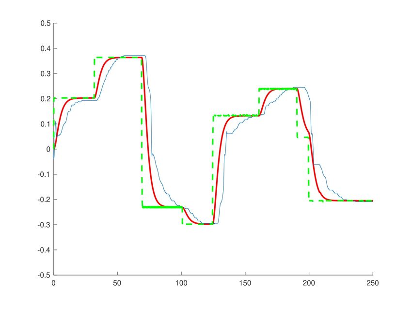
(a) PI: output variable (red), setpoint              (b) Control variable             (c) Zoom on the faults
              (black) and reference trajectory (blue)

          (d) PI: output variable (red), setpoint              (e) Control variable              (f) Zoom on the faults
              (black) and reference trajectory (blue)

          (g) PI: output variable (red), setpoint              (h) Control variable              (i) Zoom on the faults
              (black) and reference trajectory (blue)

                                                        Fig. 3: Scenarios 3, 4 & 5: MFC

          (a) PI: output variable (red), setpoint              (b) Control variable       (c) 0: no loss, 1: fault 1, 2: fault 2
              (black) and reference trajectory (blue)

                                                             Fig. 4: Scenario 2: PI

   2) Scenarios without any packet loss: Three scenarios are again considered:
 •   Scenario 4 – T = 4s.
  • Scenario 5 – T = 2s.
  • Scenario 6 – T = 0.5s.

Figures 9 and 10 display an excellent tracking for the scenarios 4 and 5. A deterioration appears in Figure 11 with respect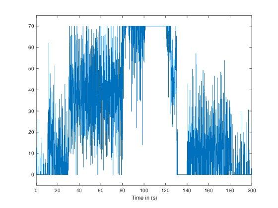
(a) PI: output variable (red), setpoint          (b) Control variable                    (c) Zoom on the faults
    (black) and reference trajectory (blue)

                                              Fig. 5: Scénario 5 : PI

(a) Output (blue), reference trajectory (b) Supply voltages v1 (blue), v2 (red) (c) Various faults: {0,1,2} = no fault,
    (red)                                                                           fault 1, fault 2

                                                Fig. 6: Scenario 1

(a) Output (blue), reference trajectory (b) Supply voltages v1 (blue), v2 (red) (c) Zoom on the faults: {0,1,2} = no
    (red)                                                                           fault, fault 1, fault 2

                                                Fig. 7: Scenario 2

(a) Output (blue), reference trajectory (b) Supply voltages v1 (blue), v2 (red) (c) Zoom on the faults: {0,1,2} = no
    (red)                                                                           fault, fault 1, fault 2

                                                Fig. 8: Scenario 3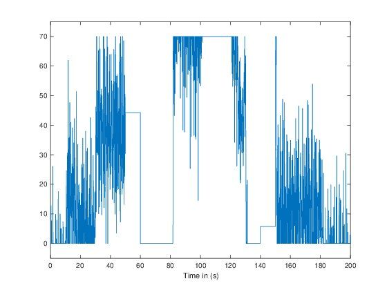
to the scenario 6: this scenario is not really feasible from a purely mechanical viewpoint. Scenario 5 seems to be the best
compromise between the speed of reaction and reachable trajectories.

                                              (a) Output (blue), reference trajectory (red), joystick (green)

                                                         (b) Supply voltages v1 (blue), v2 (red)
                                                                 Fig. 9: Scenario 4

   3) Scenarios with packet loss: Consider therefore the three following scenarios:
  • Scenario 7 – T = 2s, 2 long transmission cuts with fault 1, and 1 with fault 2;
  • Scenario 8 – T = 2s, between the supervisor and the server 23.56% of faults 1 and 25.27000% of faults 2;
  • Scenario 9 – T = 2s, between the supervisor and the server 38.79% of faults 1 and 40.50% of fault 2.
The results in Figure 12 are good outside the transmission cuts. Those in Figure 13 are quite correct in spite of an important
packet loss. The scenario 9, where the packet loss is huge, is inducing some lack of efficiency as shown in in Figure 14.
                                                                  V. C ONCLUSION
   MFC [13] might be a most promising tool for control networking. Our study corroborates [40]: “Control in the IoT imposes
control-theoretic challenges that we are unlikely to encounter in our usual application domains.” Let us stress therefore that
the robustness of MFC with respect to packet loss is today only a purely empirical fact. In the spirit of “experimental
mathematics” (see, e.g., [2]), a theoretical justification needs to be presented.
   When the transmission distance becomes large, for instance between France and USA or China, or between the Earth
and the Moon,5 latency may perhaps not be neglected anymore. A straightforward extension of our viewpoint yields to a
 5 Such   long distances might be unusual in the IIoT!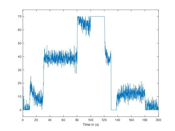
(a) Output (blue), reference trajectory (red), joystick (green)

                                               (b) Supply voltages v1 (blue), v2 (red)
                                                        Fig. 10: Scenario 5

constant delay (compare, e.g., with [12], [37], [38], [49]). In this context the approach on supply chain management in [19]
might be useful.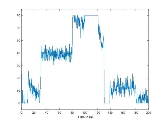
(a) Output (blue), reference trajectory (red), joystick (green)

                                         (b) Supply voltages v1 (blue), v2 (red)
                                                  Fig. 11: Scenario 6

(a) Output (blue), reference trajectory (b) Supply voltages v1 (blue), v2 (red) (c) Faults: {0,1,2} = {no fault, fault 1,
    (red), joystick (green)                                                              fault 2}

                                                  Fig. 12: Scenario 7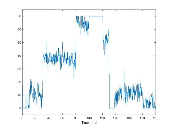
(a) Output (blue), reference trajectory (b) Supply voltages v1 (blue), v2 (red) (c) Zoom on the faults: {0,1,2} = {no
    (red), joystick (green)                                                       fault, fault 1, fault 2}

                                               Fig. 13: Scenario 8

(a) Output (blue), reference trajectory (b) Supply voltages v1 (blue), v2 (red) (c) Zoom on the faults: {0,1,2} = {no
    (red), joystick (green)                                                       fault, fault 1, fault 2}

                                               Fig. 14: Scenario 9
R EFERENCES
[1] T. Abdelzaher, Y. Hao, K. Jayarajah, A. Misra, P. Skarin, S. Yao, D.Weerakoon, K.E. Årzén. Five challenges in cloud-enabled intelligence and control.
ACM Trans. Intern. Techno., 20, 2020. https://doi.org/10.1145/3366021
[2] V.I. Arnold. Experimental Mathematics (translated from the Russian). Math. Sci. Res. Instit., 2015.
[3] K.E. Årzén, P. Skarin, W. Tärnberg, M. Kihl. Control over the edge cloud – An MPC example. 1st Int. Workshop Trustworth. Real-time Comput.
Cyber-Phys. Syst., Nashville, 2018.
[4] K.J. Åström, R.M. Murray. Feedback Systems: An Introduction for Scientists and Engineers. Princeton University Press, 2008.
[5] O. Bara, M. Fliess, C. Join, J. Day, S.M. Djouady. Toward a model-free feedback control synthesis for treating acute inflammation. J. Theoret. Biology,
448, 26-37, 2018
[6] M. Bekcheva, M. Fliess, C. Join, A. Moradi, H. Mounier. Meilleure élasticité “nuagique” par commande sans modèle. ISTE OpenSci. Contr./Automat.,
2, 15 pages, 2018. https://hal.archives-ouvertes.fr/hal-01884806/en/
[7] N. Bourbaki. Fonctions d’une variable réelle. Hermann, 1976. English translation: Functions of a Real Variable. Springer, 2004.
[8] H. Boyes, B. Hallaq, J. Cunningham, T. Watson. The industrial internet of things (IIoT): An analysis framework. Computers Industry, 101, 1-12,
2018.
[9] E.F. Camacho, C. Bordons. Model Predictive Control (2nd correct. ed.). Springer, 2007.
[10] R. Carli, G. Cavone, S. Ben Othman, M. Dotoli. IoT based architecture for model predictive control of HVAC systems in smart buildings. Sensors,
20, 2020. doi:100.27090/s20030781
[11] M. Claypool. Game input with delay–moving target selection with a game controller thumbstick. ACM Trans. Multimed. Comput. Communicat.
Appli., 14, article 57, 2018.
[12] P. Ferrari, E. Sisinni, D. Brandão, M. Rocha. Evaluation of communication latency in industrial IoT applications. Int. Workshop Measur. Network.,
Naples, 2017.
[13] M. Fliess, C. Join. Model-free control. Int. J. Contr., 86, 2228-2252, 2013.
[14] M. Fliess, C. Join, M. Bekcheva, A. Moradi, H. Mounier. A simple but energy-efficient HVAC control synthesis for data centers. 3rd Int. Conf.
Contr. Automat. Diagnos. (ICCAD’19), Grenoble, 2019. https://hal.archives-ouvertes.fr/hal-02125159/en/
[15] M. Fliess, J. Lévine, P. Martin, P. Rouchon. Flatness and defect of non-linear systems: introductory theory and examples. Int. J. Contr., 61, 1327-1361,
1995.
[16] M. Fliess, H. Sira-Ramı́rez. Closed-loop parametric identification for continuous-time linear systems via new algebraic techniques. H. Garnier & L.
Wang (Eds): Identification of Continuous-time Models from Sampled Data, Springer, pp. 362-391, 2008.
[17] A. Gilchrist. Industry 4.0: The Industrial Internet of Things. Apress, 2016.
[18] Q. Ha, M.D. Phung. IoT-enabled dependable control for solar energy harvesting in smart buildings. IET Smart Cities, 2019.
doi: 10.1049/iet-smc.270019.0052
[19] K. Hamiche, M. Fliess, C. Join, H. Abouaı̈ssa. Bullwhip effect attenuation in supply chain management via control-theoretic tools and short-term
forecasts: A preliminary study with an application to perishable inventories. 6th Int. Conf. Contr. Deci. Informat. Techno., Paris, 2019.
https://hal.archives-ouvertes.fr/hal-02050480/en/
[20] W. Han, G. Wang, A.M. Stankovic. Application of ultra-local models in automatic generation control with co-simulation of communication delay.
North Amer. Power Symp. (NAPS), Morgantown, 2017.
[21] M. Hermann, T. Pentek, B. Otto. Design principles for industrie 4.0 scenarios: A literature review. Working Paper, Technische Universität, Dortmund.
[22] C. Join, F. Chaxel, M. Fliess. “Intelligent” controllers on cheap and small programmable devices. 2nd Int. Conf. Contr. Fault-Tolerant Syst., Nice,
2013. https://hal.archives-ouvertes.fr/hal-00845795/en/
[23] C. Join, E. Delaleau, M. Fliess, C.H. Moog. Un résultat intrigant en commande sans modèle. ISTE OpenSci. Automat./Contr., 1, 9 pages, 2017.
https://hal.archives-ouvertes.fr/hal-01628322/en/
[24] C. Join, M. Fliess, F. Chaxel. Model-free control as a service and the Internet of Things (IoT): Some preliminary considerations. Tech. Rep., École
polytech., Palaiseau, 2019. https://hal.archives-ouvertes.fr/hal-02356001/en/
[25] D.-S. Kim, H. Tran-Dang. Industrial Sensors and Controls in Communication Networks – From Wired Technologies to Cloud Computing and Internet
of Things. Springer, 2019.
[26] C. Korte, S.S. Nair, V. Nistor, T.P. Low, C.R. Doarn, G. Schaffner. Determining the threshold of time-delay for teleoperation accuracy and efficiency
in relation to telesurgery. Telemed. e-Health, 20, 1078-1086, 2014.
[27] R. Kouki, A. Boe, T. Vantroys, F. Bouani. IoT predictive application for DC motor control using radio frequency links. Medit. Microwave Symp.,
Marseille, 2017.
[28] R. Kouki, A. Boe, T. Vantroys, F. Bouani. Autonomous Internet of Things predictive control application based on wireless networked multi-agent
topology and embedded operating system. J. Syst. Contr. Engin., 234, 577-595, 2020
[29] S. Kumar, S. Rai. Survey on transport layer protocols: TCP & UDP. Int. J. Comput. App., 46, 20-25, 2012.
[30] J.F. Kurose, K.W. Ross. Computer Networking (5th ed.). Addison-Wesley, 2010.
[31] F. Lafont, J.-F. Balmat, N. Pessel, M. Fliess. A model-free control strategy for an experimental greenhouse with an application to fault accommodation.
Comput. Electron. Agricul., 110, 139-149, 2015.
[32] X.F. Liu, M.R. Shahriar, S.M.N. Al Sunny, M.C. Leub, L. Hub. Cyber-physical manufacturing cloud: Architecture, virtualization, communication,
and testbed. J. Manufact. Syst., 43, 352-364, 2017.
[33] M.S. Mahmoud, Y. Xia. Networked Control Systems – Cloud Control and Secure Control, Butterworth-Heinemann, 2019.
[34] S. Manfredi. Multilayer Networked Control of Cyber-physical Systems. Springer, 2017.
[35] D.C. Marinescu. Cloud Computing – Theory and Practice. Morgan Kaufmann, 2013.
[36] T.F. Megahed, S.M. Abdelkader, A. Zakaria. Energy management in zero-energy building using neural network predictive control. IEEE Internet
Things J., 6, 5336-5344, 2019.
[37] V. Millnert. A Timely Journey Through the Cloud. Ph.D. Thesis, Dept. Automat. Contr., Lunds Universitet, 2019.
[38] V. Millnert, J. Eker, E. Bini. Achieving predictable and low end-to-end Latency for a network of smart services. IEEE Glob. Communicat. Conf.
(GLOBECOM), Abu Dhabi, 2018.
[39] P. Prouvost. Automatique – Contrôle et régulation (2e éd.) Dunod, 2010.
[40] T. Samad. Control systems and the Internet of Things. IEEE Contr. Syst. Magaz., 36, 13-16, 2016.
[41] T. Schulz (Hrsg.). Industrie 4.0: Potenziale erkennen und umsetzen. Vogel Business Media, 2017.
[42] W.McC. Siebert. Circuits, Signals and Systems. MIT Press, 1986.
[43] H. Sira-Ramı́rez, C. Garcı́a-Rodrı́guez, J. Cortès-Romero, A. Luviano-Juárez. Algebraic Identification and Estimation Methods in Feedback Control
Systems. Wiley, 2014.
[44] P. Skarin, J. Eker, M. Kihl, Karl-Erik Årzén. An assisting model predictive controller approach to control over the cloud.
arXiv:1905.06305, 2019
[45] Suberman, Suwendri, M. Al-Akaidi. A review on transport layer protocol performance for delivering video on an adhoc network. IOP Conf. Ser.
Mater. Sci. Engin., 237, 0120018, 2017.[46] C.C. Wu, K.T. Chen, C.M. Chen, P. Huang, C.L. Lei. On the challenge and design of transport protocols for MMORPGs. Multimed. Tools Appl.,
45, 7-32, 2009.
[47] A. Vick, J. Guhl, J. Kruger. Model predictive control as a service - concept and architecture for use in cloud-based robot control. 21st Int. Conf.
Meth. Models Automat. Robot., Miedzyzdroje 2016.
[48] Y.-Q. Xia, Y.-L. Gao, L.-P. Yan, M.-Y. Fu. Recent progress in networked control systems – A survey. Int. J. Automat. Comput., 12, 343-367, 2015.
[49] A.A. Yaseen, M. Bayart. A model-free approach to networked control system with time-varying communication delay. IFAC-PapersOnLine, 51-24,
558-563, 2018.
[50] K. Yosida. Operational Calculus (translated from the Japanese). Springer, 1984.
[51] Y. Zitelli, F. Tao. Optimization of Manufacturing Systems Using the Internet of Things Academic Press, 2017.You can also read