Lora RTT Ranging Characterization and Indoor Positioning System - Hindawi.com

Page created by Christian Campbell
 
CONTINUE READING
Lora RTT Ranging Characterization and Indoor Positioning System - Hindawi.com
Hindawi
Wireless Communications and Mobile Computing
Volume 2021, Article ID 5529329, 10 pages
https://doi.org/10.1155/2021/5529329

Research Article
Lora RTT Ranging Characterization and Indoor
Positioning System

         Qiang Liu,1 XiuJun Bai,2 Xingli Gan ,3 and Shan Yang2
         1
           CHN Energy, Huanghua Port Affairs Co. Ltd, Cangzhou, Hebei, China
         2
           China Unicom Smart City Research Institute, Baoding, Hebei, China
         3
           Zhejiang University of Science and Technology, Hangzhou, Zhejiang, China

         Correspondence should be addressed to Xingli Gan; ganxingli@163.com

         Received 10 January 2021; Revised 29 January 2021; Accepted 8 February 2021; Published 3 March 2021

         Academic Editor: Liangtian Wan

         Copyright © 2021 Qiang Liu et al. This is an open access article distributed under the Creative Commons Attribution License,
         which permits unrestricted use, distribution, and reproduction in any medium, provided the original work is properly cited.

         In recent years, indoor positioning systems (IPS) are increasingly very important for a smart factory, and the Lora positioning
         system based on round-trip time (RTT) has been developed. This paper introduces the ranging characterization, RTT
         measurement, and position estimation method. In particular, a particle filter localization method-aided Lora pseudorange fitting
         correction is designed to solve the problem of indoor positioning; the cumulative distribution function (CDF) criteria are used
         to measure the quality of the estimated location in comparison to the ground truth location; when the positioning error on the x
         -axis threshold is 0.2 m and 0.6 m, the CDF with pseudorange correction is 61% and 99%, which are higher than the 32% and
         85% without pseudorange correction. When the positioning error on the y-axis threshold is 0.2 m and 0.6 m, the CDF with
         pseudorange correction is 71% and 99.9%, which are higher than the 52% and 94.8% without pseudorange correction.

1. Introduction                                                       provides ultra-long-range communication in the 2.4 GHz
                                                                      band with a time-of-flight functionality; its radio is fully
Indoor positioning systems are increasingly very important            compliant with all worldwide 2.4 GHz radio regulations
for a smart factory, such as finding the location of workers,          including EN 300440, FCC CFR 47 Part 15 [19], and the Jap-
goods, or vehicles [1–4]. However, the Global Positioning             anese ARIB STD-T66 [20]. Very small wearable products to
System (GPS) is unable to provide the indoor positioning ser-         track and localize assets in logistic chains and people for
vice, which is commonly used for outdoor positioning. The             safety can easily be designed thanks to the high level of inte-
research on indoor positioning technologies has been con-             gration and the ultralow current consumption which allows
ducted for more than three decades, such as Radio Frequency           the use of miniaturized batteries.
Identification (RFID) [5, 6], WiFi [7, 8], Ultra Wide Band                 But the most difficult challenge for Lora indoor position-
(UWB) [9–11], Pseudolite [12–14], Bluetooth [15], and Iner-           ing is the ranging error caused by multipath in the indoor
tial Navigation System (INS), but they may not be suitable for        environment. Liang et al. carry out the study focused on the
Internet of Things (IoT) applications in terms of cost, appli-        indoor propagation of the Lora signal, and the main contri-
cation mode, and terminal power consumption.                          bution of this work is to measure the round-trip time and
     With the continuous progress of sensor and Internet of           packet delivery ratio by changing send power, payload
Things [16, 17] technologies, increasing attention has been           length, and air rate in a multilevel building from the 1st floor
paid to IPS using Lora WAN. Semtech has developed a Lora              to the 12th floor [21]. Huynh and Brennan verify the UWB
positioning system based on round-trip time [18], which is            transmission characteristics of an indoor RTT signal by gen-
called the SX1280 transceiver. The SX1280 transceiver family          erating synthetic received signals using ray tracing plus
Lora RTT Ranging Characterization and Indoor Positioning System - Hindawi.com
2                                                                                   Wireless Communications and Mobile Computing

Rayleigh distributed random multipath clusters as well as                                                  Tround
random amplitude and delay factors [22]. Staniec and Kowal               Lora_A                                                                   time
describe outcomes of measurement campaigns during which
                                                                             Tx_A                                           Rx_A
the Lora performance was tested against a heavy multipath
propagation and a controlled [23], Lora configurational
space is divided into three distinct sensitivity regions: in the
white region, it is immune to both interference and multipath
propagation; in the light-grey region, it is only immune to the
multipath phenomenon but sensitive to interference; and in                            RAB                                RBA
the dark grey region, Lora is vulnerable to both phenomena.
     On the other hand, location based on a filtering algorithm                                                          Tx_B
                                                                         Lora_B        Rx_B                                                    time
is the only effective solution currently known, and the Bayes-
ian filtering algorithm occupies an important role. In the                                                  Treply
early days, the Kalman filter positioning algorithm is mainly
used to solve the problem achieving efficient state estimation                         Figure 1: RTT measurement illustration.
for linear Gaussian systems [24]. Moreover, to deal with
unwanted errors and nonlinear distortions, particle filter
(PF) is applied as a nonparametric filter to location, which
is recursive implementations of Monte Carlo-based statistical                                   Z
                                                                                                                     AP3
processing [25–27] and performs well in localization effi-                                AP2                       (x3, y3, z3)
ciency, stability, and accuracy.                                                     (x2, y2, z2)
     In the following sections, a Lora indoor positioning sys-                                                                             AP4
                                                                               AP1
tem is introduced, which overcomes the problem of long dis-                                                                             (x4, y4, z4)
                                                                            (x1, y1, z1)
tance, low power consumption, and low cost. The main
contributions and research content of this paper are as fol-
lows: Firstly, a Lora-aided particle filter localization method                                                                                           Y
is designed to solve the problem of indoor positioning. Sec-
ondly, numerous experiments were carried out with real Lora
RTT measurement data to evaluate the performance of the                                                                    User
proposed approach; we used the CDF criteria to measure                                                                   (x, y, z)
the quality of the estimated location in comparison to the                      X
ground truth location. The results show that the indoor posi-
                                                                     Figure 2: Position estimation by four distance measurements.
tioning accuracy is improved obviously with the help of the
piecewise fitting correction method. At the same time, the
Lora indoor positioning system can achieve a positioning                If the clock characteristics of Lora_A and Lora_B are sta-
accuracy of 1 m under the condition of LOS.                        ble, t r A = t s A and t r B = t s B at the adjacent time of receiving
                                                                   and transmitting. The time-of-flight (ToF) measurements
2. Background and Related Work                                     can be written as
2.1. Lora RTT Measurement. In this paper, we focus on one of
the latest techniques called the RTT scheme-based ranging            T round = ρAB + T reply + ρBA = RAB + RBA + t r                       B
and localization [28–30], which can give accurate measure-                           − ts       + tr       − ts         + T reply = RAB + RBA + T reply ,
                                                                                            A          A            B
ments by the time stamp from the initiator (Lora_A) to the
responder (Lora_B) with nanosecond resolution. Figure 1                                                                                                      ð3Þ
shows the RTT measurement illustration; the pseudorange
measurement can be built as                                        where T round is the time-of-flight (ToF) measurements of
                                                                   Lora_A from Tx_A to Rx_A, T reply is the time difference of
                    ρAB = RAB + t r     A   − ts B,         ð1Þ    Lora_B between Rx_B and Tx_B.
                                                                      The geometric distance can be calculated by

                                                            ð2Þ                                                                  
                  ρBA = RBA + t r   B   − ts A ,                                                                 T round ‐T reply
                                                                                                 RAB =                              :                        ð4Þ
                                                                                                                        2
where ρAB or ρBA is the pseudorange measurement between
Lora_A and Lora_B, RAB or RBA is the geometric range                    The pseudorange measurement can be built as
between Lora_A and Lora_B, t r A is the clock offset of
Lora_A at the receiving time, t s A is the clock offset of                                 qffiffiffiffiffiffiffiffiffiffiffiffiffiffiffiffiffiffiffiffiffiffiffiffiffiffiffiffiffiffiffiffiffiffiffiffiffiffiffiffiffiffiffiffiffiffiffiffiffiffiffiffiffiffiffiffiffiffiffiffiffiffiffiffiffiffiffiffi
                                                                         T round ‐T reply
Lora_A at the transmitting time, t r B is the clock offset of       RAB =                   = ðxA − xB Þ2 + ðyA − yB Þ2 + ðz A − z B Þ2 + ε,
Lora_B at the receiving time, and t s B is the clock offset of                   2
Lora_B at the transmitting time.                                                                                                                             ð5Þ
Lora RTT Ranging Characterization and Indoor Positioning System - Hindawi.com
Wireless Communications and Mobile Computing                                                                                                                                                                   3

                                                                             Table 1: Relationship between ranging error, clock error, and flight time.
                                                                  
Clock error T reply + RAB                                                                0.1 ppm                   0.5 ppm                                5 ppm                                     25 ppm
                                                                                                 −4                      −4                                      −3
1.5 μs                                                                                1:5 × 10 ns                7:5 × 10 ns                         7:5 × 10 ns                               3:75 × 10−2 ns
10 μs                                                                                 1:5 × 10⁻³ ns              7:5 × 10⁻³ ns                       7:5 × 10⁻² ns                             3:75 × 10−1 ns
100 μs                                                                                1:5 × 10⁻² ns              7:5 × 10⁻² ns                       7:5 × 10⁻¹ ns                                  3:75 ns
                                                                                                 −1                      −1
1000 μs                                                                               1:5 × 10 ns                7:5 × 10 ns                              7:5 ns                                    37:5 ns
10000 μs                                                                                     1:5 ns                 7:5 ns                                 75 ns                                     375 ns

                                    2
                                                                                                                   (xu , yu , z u ) can be calculated by
                                    0                                                                                  8        qffiffiffiffiffiffiffiffiffiffiffiffiffiffiffiffiffiffiffiffiffiffiffiffiffiffiffiffiffiffiffiffiffiffiffiffiffiffiffiffiffiffiffiffiffiffiffiffiffiffiffiffiffiffiffiffiffiffiffiffiffiffiffiffiffiffi
                                                                                                                       >
                                                                                                                       >         ðx1 − xu Þ2 + ðy1 − yu Þ2 + ðz 1 − zu Þ2 + ε1u ,
                                                                                                                       > 1u
                                                                                                                         R    =
    Ranging error (s)

                                                                                                                       >
                                                                                                                       >
                                                                                                                       >
                                                                                                                       >        qffiffiffiffiffiffiffiffiffiffiffiffiffiffiffiffiffiffiffiffiffiffiffiffiffiffiffiffiffiffiffiffiffiffiffiffiffiffiffiffiffiffiffiffiffiffiffiffiffiffiffiffiffiffiffiffiffiffiffiffiffiffiffiffiffiffi
                                                                                                                       >
                                                                                                                       >
                         −2                                                                                            >
                                                                                                                       < R2u = ðx2 − xu Þ2 + ðy2 − yu Þ2 + ðz 2 − zu Þ2 + ε2u ,
                                                                                                                       >        qffiffiffiffiffiffiffiffiffiffiffiffiffiffiffiffiffiffiffiffiffiffiffiffiffiffiffiffiffiffiffiffiffiffiffiffiffiffiffiffiffiffiffiffiffiffiffiffiffiffiffiffiffiffiffiffiffiffiffiffiffiffiffiffiffiffi
                                                                                                                       >
                                                                                                                       >
                                                                                                                       >
                                                                                                                       > R 3u =  ðx3 − xu Þ2 + ðy3 − yu Þ2 + ðz 3 − zu Þ2 + ε3u ,
                         −4                                                                                            >
                                                                                                                       >
                                                                                                                       >
                                                                                                                       >        qffiffiffiffiffiffiffiffiffiffiffiffiffiffiffiffiffiffiffiffiffiffiffiffiffiffiffiffiffiffiffiffiffiffiffiffiffiffiffiffiffiffiffiffiffiffiffiffiffiffiffiffiffiffiffiffiffiffiffiffiffiffiffiffiffiffi
                                                                                                                       >
                                                                                                                       : R = ð x − x Þ2 + ðy − y Þ 2 + ðz − z Þ2 + ε ,
                                                                                                                           4u        4        u              4       u              4        u      4u
                         −6
                                                0                      10               20                 30                                                                                                 ð6Þ
                                                                        True distance (m)
                                                                                                                   where Riu is the pseudorange measurement of APi , i is the AP
                                                          Test1
                                                          Test2                                                    index, and u is the user index, (xi , yi , z i ) are the locations of
                                                          Test3                                                    APi , and εiu is the measurement error of APi .
                                                                                                                       The geometric distance can be calculated by
                                                        Figure 3: Ranging error under LOS.
                                                                                                                                     ðx − x i Þx u + ðy u − y i Þ y u + ðz u − z i Þ z u
                                      10                                                                                       Riu = quffiffiffiffiffiffiffiffiffiffiffiffiffiffiffiffiffiffiffiffiffiffiffiffiffiffiffiffiffiffiffiffiffiffiffiffiffiffiffiffiffiffiffiffiffiffiffiffiffiffiffiffiffiffiffiffiffiffiffiffiffiffiffi
                                                                                                                                                                                                     ffi
                                            8
                                                                                                                                        ð x i − x u Þ2 + ð y i − y u Þ2 + ð z i − z u Þ2
                                                                                                                                                                  2 3
                                            6
                                                                                                                                                                      xu                                      ð7Þ
                        Ranging error (s)

                                                                                                                                               h                i6 7
                                            4                                                                                        + εiu = eix , eiy , eiz 6              7
                                                                                                                                                                  6 yu 7 + εiu ,
                                                                                                                                                                  4 5
                                            2                                                                                                                          zu
                                            0

                                    −2
                                                                                                                   where ½eix , eiy , eiz  is called a geometry matrix.
                                                                                                                       The observation equations of Lora RTT can be expressed
                                    −4                                                                             as the following matrix form:
                                                    0                  10               20            30
                                                                        True distance (m)
                                                                                                                                 2     3 2 1  e1  1 3      2 3
                                                                                                                                     R1u     ex  y  ez 2 3     ε1u
                                                           Test1
                                                                                                                                 6     7 6         7 xu      6     7
                                                           Test2                                                                           6        2      7
                                                                                                                                 6 R2u 7 6 e2  ey  e2 76 7 6 ε2u 7
                                                           Test3                                                                 6     7 = 6 x   z 76 7 + 6 7:                                              ð8Þ
                                                                                                                                 6     7           74 y u 5 6      7
                                                                                                                                 6⋮7 6       e3x  e3y  e3z 7 6⋮7
                                                        Figure 4: Ranging error under NLOS.                                      4     5 6 4   5 zu          4     5
                                                                                                                                               4 4 4
                                                                                                                                   R4u       ex  e  ez         ε4u
                                                                                                                                                           y

where xA , yA , and z A are the transmitting antenna coordi-
nates of Lora_A; xB , yB , and z B are the transmitting antenna                                                       The matrix on the right-hand side of Equation (8) is
coordinates of Lora_B; and ε is measurement error.                                                                 defined as A and ε, and the two-column vectors on the left-
                                                                                                                   hand side are defined as b. Equation (8) can be written as

2.2. Position Estimation. Four distance measurements of Lora                                                                                             b = AX + ε:                                          ð9Þ
transceivers whose positions are known are used to deter-
mine the three-dimensional coordinates of an unknown                                                                  If an initial value X 0 is used for the solution-updating
position [31], as shown in Figure 2. The position of user                                                          process, the Newton-Raphson method is described
Lora RTT Ranging Characterization and Indoor Positioning System - Hindawi.com
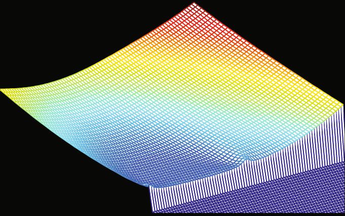
4                                                                                                                          Wireless Communications and Mobile Computing

                                           40                                                                 0.997
                                                                                                               0.99
                                                                                                               0.98
                                                                                                               0.95
                                           30                                                                  0.90
                                                                                                               0.75

                                                                                                Probability
                                  Number

                                           20                                                                  0.50
                                                                                                               0.25
                                           10                                                                  0.10
                                                                                                               0.05
                                                                                                               0.02
                                                                                                               0.01
                                           0
                                                                                                              0.003
                                                0    −5            0            5         10
                                                                Ranging error                                         −5                    0               5
                                                                                                                                          Ranging error (m)
                                                    Ranging error
                                                    norm fit
                                                                     (a)                                                                    (b)

                                      Figure 5: Probability characterization: (a) histogram with a distribution fit and (b) normal probability plot.

                          2                                                                                                    Lora4 (0, 40, 3)                 Lora3 (40, 40, 3)
                                                                                                                           Z

                          0
     Ranging error (s)

                                                                                                                               Lora 1 (0, 0, 3)
                         −2                                                                                                                                     Lora2 (40, 0, 3)
                                                                                                                                                         Y

                         −4                                                                                                                       User

                                                                                                                                                                             X
                         −6
                              0                      10                20           30
                                                       True distance (m)                                          Figure 7: Simulation conditions of geometry distribution.
                                           Test1
                                           Test2
                                           Test3
                                                                                                              tion of ranging error is as follows:
                              Figure 6: Piecewise linear fitting correction.
                                                                                                                                          ðεA − εB Þ              
                                                                                                                                   εt =             × T reply + RAB ,               ð12Þ
asX 0 = ðxu,0 , yu,0 , z u,0 Þ. The least-squares updated solution                                                                            2
can be represented as
                                                                                                              where εt is ranging error caused by the clock offsets.
                                                             −1                                                If the clock error of Lora_A and Lora_B is the same,
                                                ΔX = A A  T
                                                                    A b + ε:
                                                                     T
                                                                                         ð10Þ
                                                                                                              Equation (12) can be written as
    Then, the position X 1 can be updated iteratively accord-                                                                                                 
ing to                                                                                                                                  εt = εA × T reply + RAB :                   ð13Þ

                                                    X 1 = X 0 + ΔX:                      ð11Þ                     It is supposed that the distance between the two Lora
                                                                                                              nodes is between 10 meters and 5000 meters; then, RAB is
    It should be noted that the measurement error is consid-                                                  from 3 ns to 1500 ns. The clock error of packaged crystal
ered Gaussian white noise, when using the least-squares                                                       oscillator (PCO) is generally more than 25 ppm, the temper-
method.                                                                                                       ature compensated crystal oscillator (TCXO) is from 0.5 ppm
                                                                                                              to 5 ppm, and the oven-controlled crystal oscillator (OCXO)
3. Ranging Characterization of Lora                                                                           may be less than 0.1 ppm. According to the above parame-
                                                                                                              ters, we estimate the influence of clock error on Lora ranging
3.1. Clock Error. It is supposed that the clock offsets of devices                                             accuracy, as shown in Table 1. It can be found that TCXO
Lora_A and Lora_B are εA and εB ; therefore, the ranging                                                      and OCXO are best used as the clock of the Lora positioning
error will increase with the increase of flight time. The equa-                                                system.
Lora RTT Ranging Characterization and Indoor Positioning System - Hindawi.com
Wireless Communications and Mobile Computing                                                                                                                                      5

                     1.5                                                                     1.5

                      1                                                                          1
                 z                                                                       z
                     0.5                                                                     0.5

                      0                                                                       0
                     40                                                                      40
                                                                                    40                                                                             40
                                    20                                                                     20
                                                                      20                                                                               20
                                     y            0     0             x                                        y            0    0                 x
                                                      (a)                                                                       (b)

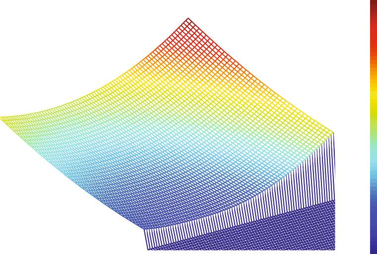
       Figure 8: Indoor positioning system composed of four Lora transceivers: (a) HDOP and (b) GDOP in the projection area.

                                                                                                                                                                        6
             6                                                                               8
                                                                                    3                                                                                   5
                                                                                             6
             4
                                                                                                                                                                        4
         z                                                                          2    z 4
             2                                                                                                                                                          3
                                                                                             2

           0                                                                               0                                                                            2
                                                                                    1
          80                                                                              80
                                                                               80                                                                                  80   1
                           60                                             60
                                                                          60                              60                                                60
                                                                                                                                                            60
                                                                 40
                                                                 40                                                                                40
                                                                                                                                                   40
                                                        20                          0                                                     20                            0
                                y        40   0              x                                                 y       40       0              x
                                                  (a)                                                                               (b)

     Figure 9: Indoor positioning system composed of four Lora transceivers: (a) HDOP and (b) GDOP outside the projection area.

3.2. Ranging Accuracy and Characterization. The reflection                                      In order to analyze the distribution characteristics of Lora
of the indoor environment to the Lora positioning signal is                               ranging error, the six groups of data collected above are com-
very serious, for example, irregular room structure, walking                              bined, as shown in Figure 5. Figure 5(a) shows the histogram
people, tables and chairs, and glass. Because of signal inter-                            with a distribution fit, and Figure 5(b) is the normal probabil-
ference and multipath effect, Lora’s ranging error may be                                  ity plot. It can be concluded that the probability distribution
non-Gaussian distribution. We collect the ranging data of                                 of Lora ranging error is non-Gaussian white noise. Therefore,
Lora under different conditions such as line-of-sight (LOS),                               it is necessary to use nonlinear filter to solve the location
non-line-of-sight (NLOS), and human occlusion, which is                                   problem.
compared with the real distance to analyze the ranging                                         The piecewise fitting correction method of LOS is used to
characterization.                                                                         correct the Lora ranging value, as shown in Figure 6. The for-
     Three sets of ranging data are collected under the LOS                               mula of the piecewise fitting correction method can be
condition; the ranging error of Lora is shown in Figure 3.                                expressed as
The average error is -0.61 m, the maximum error is 1.2 m,
                                                                                                                                    _
and the minimum error is -5.24 m. It can be found that the                                                                          R = R + f ðRÞ,                              ð14Þ
ranging error of LOS has a linear trend, which can be cor-
rected by the polynomial fitting method.                                                                        8
                                                                                                               >
                                                                                                               > a + a11 × R,              0 ≤ R ≤ r1 ,
     Similarly, three sets of ranging data are collected under                                                 > 10
                                                                                                               >
                                                                                                               >
                                                                                                               < a20 + a21 × R,
the NLOS condition, such as using people’s bodies to block                                                                                 r1 < R ≤ r2 ,
Lora’s antenna; the ranging error of Lora is shown in                                                f ðRÞ =                                                                    ð15Þ
                                                                                                               >
                                                                                                               >                                                    ⋮
Figure 4. The average error is -0.01 m, the maximum error                                                      >
                                                                                                               >
                                                                                                               >
                                                                                                               :
is 8.6 m, and the minimum error is -3.32 m. It can be found                                                        am0 + am1 × R,              r m−1 < R ≤ r m ,
that the ranging error of NLOS is much worse than that of
                                                                                                                                                                            _
LOS; therefore, it is better to use the Lora indoor positioning                           where R is the pseudorange measurement of Lora, R is the
system under the condition of LOS.                                                        corrected pseudorange, f ðRÞ is the correction function, a10
Lora RTT Ranging Characterization and Indoor Positioning System - Hindawi.com
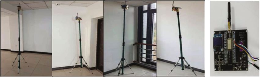
6                                                                                          Wireless Communications and Mobile Computing

                                                         Table 2: Particle filter algorithm.

Process                                                                                  Content
Initialization                                                        Let X i1 ~ pðX 0 Þ, i = 1, ⋯, N, and wi0 = 1/N
Iteration
                                                                                                                                                        
(1) Measurement update           For i = 1, ⋯, N, wit = ð1/ct Þwit−1 p Y t /X it , where the normalization weight is given by ct = ∑Nt=1 wit−1 p Y t /X it
                                                                                                                         
(2) Estimation                               The filtering density is approximated by pðX t /Y t Þ ≈ ∑Ni=1 wit δ X t − X it ,X t ≈ ∑Ni=1 wit X it
                                                                                                                                  N
                                          Optionally at each time, take N samples with replacement from the set X it , wit i=1 , where
(3) Resampling
                                                               the probability to take sample i is wit and let wit = 1/N
                                                                                                                                        
                                            Generate predictions according to the proposal distribution: X it+1 ~ q X t+1 /X it , Y t+1 , and
(4) Time update                                                                                                                      
                                                compensate for the importance weight wit+1 = wit p X it+1 /X it /q X it+1 /X it , Y t+1

                2.5m

                          AP1                                                                                                         AP3

                                                                  User
                                                                                                                                             4m

                       AP2
                                                                                                           AP4

                                                                     25 m

                       AP1                    AP2                        AP3                    AP4                            User

                                  Figure 10: Experimental environment of Lora indoor positioning system.

and a11 are the linear correction factors, and r m−1 and r m are               as follows:
the stages; the above data of LOS are divided into three sec-
tions; that is, m = 3.                                                                             2                                          3
                                                                                                       xDOP2
                                                                                               6                                              7
                                                                                             H=6
                                                                                               4                      yDOP2                   7:
                                                                                                                                              5        ð17Þ
3.3. Geometry Factor. The dilution of geometry precision
(GDOP) [32, 33] can be expressed as                                                                                                   zDOP2

                                            −1                                    HDOP and GDOP can be defined as
                       cov ðΔX Þ = σ2ε ⋅ AT A :                     ð16Þ

                                                                                                        qffiffiffiffiffiffiffiffiffiffiffiffiffiffiffiffiffiffiffiffiffiffiffiffiffiffiffiffiffiffiffiffiffi
                  −1                                                                       HDOP =        xDOP2 + yDOP2 ,                               ð18Þ
    If ðA AÞ is defined as H, the diagonal elements of H are
            T
Lora RTT Ranging Characterization and Indoor Positioning System - Hindawi.com
Wireless Communications and Mobile Computing                                                                                                                                           7

                      4 4                                                                     3                  0.5

                      3                                                                                            0

                                                                                                    Error (m)
              y (m)

                      2                     1                                                                   −0.5

                      1                                                                                           −1

                      0 1                                                                      2                   0
                        0              5            10                    15        20        25                       0            50             100       150            200
                                                         x (m)                                                                                   Time (s)
                                                       (a)                                                                                   (b)

                                                                          0.6

                                                                          0.4
                                                             Error (m)

                                                                          0.2

                                                                           0

                                                                         −0.2

                                                                         −0.4

                                                                         −0.6
                                                                                0        50           100                     150          200
                                                                                                    Time (s)
                                                                                                   (c)

Figure 11: Static test without pseudorange correction: (a) positioning results, (b) x-axis positioning error, and (c) y-axis positioning error.

                          qffiffiffiffiffiffiffiffiffiffiffiffiffiffiffiffiffiffiffiffiffiffiffiffiffiffiffiffiffiffiffiffiffiffiffiffiffiffiffiffiffiffiffiffiffiffiffiffiffiffiffi                                  tion to compute the posterior distribution is given by
          GDOP =           xDOP2 + yDOP2 + zDOP2 ,                                        ð19Þ
                                                                                                                           8         ð              
                                                                                                                           >     Xt           Xt         X t−1
where xDOP2 means the dilution of precision (DOP)                                                                          >
                                                                                                                           > p      =   p           p           dX t−1 ,
                                                                                                                           < Y t−1          X t−1        Y t−1
for the x-coordinate and yDOP2 means the DOP for                                                                                                                                 ð20Þ
the y-coordinate.                                                                                                          >
                                                                                                                           >    X   pðyt /X t ÞpðX t /Y t−1 Þ
                                                                                                                           >
                                                                                                                           :p t =                             ,
    In order to analyze the influence of the geometry factor                                                                     Yt       pðyt /Y t−1 Þ
on Lora positioning performance, a simulation of geometry
distribution is designed, which is composed of four Lora
transceivers. Suppose the length and width of the room are                                                      where t is the time stamp, xt is the state variable, pðX t‐1 /Y t‐1 Þ
40 meters and the height is 3 meters, as shown in Figure 7.                                                     is the posterior probability distribution of the last moment,
The HDOP of the indoor positioning system is given in                                                           pðX t /X t‐1 Þ is the state transition probability, pðX t /Y t‐1 Þ is
Figures 8(a) and 9(a); the GDOP of the indoor positioning                                                       the prior probability distribution, pðyt /X t Þ is the likelihood
system is given in Figures 8(b) and 9(b). The results show                                                      function, and pðyt /Y t−1 Þ is the normalization function.
that four Lora transceivers can obtain the suitable geometric                                                                                                                      N
distribution in their projection area, whose HDOP and G                                                         4.2. Particle Filter. Supposed that N particles fX it , wit gi=1
DOP are less than 1.2. However, outside the projection area,                                                    from the posterior probability pðX t /Y t Þ of the state can be
the geometric distribution will deteriorate; HDOP and G                                                         extracted, where X it is the state of the particle, wit is the weight
DOP will be greater than 2, which will make the positioning                                                     of the particle; then,
error more than twice of the ranging error.
                                                                                                                                          
4. Methodology Based on Particle Filter                                                                                                     X        N
                                                                                                                                                                      
                                                                                                                                         p t       ≈ 〠 wit δ X t − X it ,         ð21Þ
                                                                                                                                            Yt        i=1
4.1. Recursive Bayesian Estimation. Applied nonlinear filter-
ing is based on discrete-time nonlinear state-space models
relating a hidden state X t to the observations Y t , denote the                                                where δ is the Dirac delta function and N is the number of
observations at time t by Y t = fy0 , ⋯, yt g, the Bayesian solu-                                               particles.
Lora RTT Ranging Characterization and Indoor Positioning System - Hindawi.com
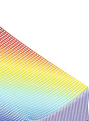
8                                                                                                                          Wireless Communications and Mobile Computing

                       4 4                                                                      3
                                                                                                                 0.4
                       3                                                                                         0.2

                                                                                                    Error (m)
                                                                                                                   0
               y (m)

                       2                       1
                                                                                                                −0.2

                       1                                                                                        −0.4

                                                                                                                −0.6
                       0 1                                                                      2
                         0                 5         10                   15         20        25               −0.8
                                                                                                                       0         50       100        150        200
                                                          x (m)
                                                                                                                                        Time (s)
                                                        (a)                                                                            (b)

                                                                           0.4

                                                                           0.2
                                                              Error (m)

                                                                            0

                                                                          −0.2

                                                                          −0.4

                                                                          −0.6

                                                                          −0.8
                                                                                 0        50            100                150        200
                                                                                                      Time (s)
                                                                                                    (c)

    Figure 12: Static test with pseudorange correction: (a) positioning results, (b) x-axis positioning error, and (c) y-axis positioning error.

   The Sequential Importance Sampling (SIS) method is                                                           steps, which includes measurement update, estimation,
used to calculate the weight of particles, which is written as                                                  resampling, and time update.
                                                                  
                                          p Y t /X it p X it /X it−1                                            5. Experimental Results and Analysis
                       wit   = wit−1                              :                      ð22Þ
                                             q X it /X it−1 , Y t
                                                                                                                5.1. Experimental Setup. The performance of the Lora posi-
                                                                                                                tioning system is evaluated in a room as shown in
    The prior probability distribution is used as the impor-                                                    Figure 10; the size of the room is about 25 meters long, 4
tance density function:                                                                                         meters wide, and 2.5 meters high; and the antenna coordi-
                                                                                                                nates of Lora are surveyed precisely with a total station.
                                                       
                                      X it                 X it
                             q              , Yt   =p            :                         ð23Þ                 5.2. Experimental Results. Figure 11 shows the static test
                                     X it−1               X it−1
                                                                                                                without pseudorange correction for the Lora positioning sys-
                                                                                                                tem, Figure 11(a) is the positioning results, Figure 11(b) is the
      Then, the formula for calculating the weight of particles is                                              x-axis positioning error, and Figure 11(c) is the y-axis posi-
                                                                                                               tioning error. The average positioning error is 0.11 m in the
                                                     Y                                                          x-axis and 0.07 m in the y-axis, the maximum positioning
                                      wit = wit−1 p ti ,                                   ð24Þ
                                                     Xt                                                         error is 1.25 m in the x-axis and 0.59 m in the y-axis, and
                                                                                                                the standard deviation of the x-axis and y-axis errors is
where t is time stamp, i is the number of particles, and w is                                                   0.42 m and 0.18 m, respectively.
the weight of particles.                                                                                            Figure 12 shows the static test without pseudorange cor-
                                                                                                                rection (the piecewise fitting correction method) for the Lora
4.3. Particle Filter Implementation. The particle filter algo-                                                   positioning system, Figure 12(a) is the positioning results,
rithm is summarized in Table 2. Firstly, the state parameters                                                   Figure 12(b) is the x-axis positioning error, and
and weights of particles are initialized; secondly, the iterative                                               Figure 12(c) is the y-axis positioning error. The average posi-
process of the particle filter algorithm is divided into four                                                    tioning error is 0.01 m in the x-axis and 0.07 m in the y-axis,
Lora RTT Ranging Characterization and Indoor Positioning System - Hindawi.com
Wireless Communications and Mobile Computing                                                                                                  9

                    1                                                           1

                   0.8                                                         0.8

                   0.6                                                         0.6

                                                                         CDF
             CDF

                   0.4                                                         0.4

                   0.2                                                         0.2

                    0                                                           0
                         0             0.5                  1                        0          0.2            0.4         0.6
                                      Positioning error (m)                                       Positioning error (m)

                             with pseudo-range correction                                with pseudo-range correction
                             without pseudo-range correction                             without pseudo-range correction

                                            (a)                                                        (b)

                                  Figure 13: Comparison of CDF positioning errors: (a) x-axis and (b) y-axis.

the maximum positioning error is 0.72 m in the x-axis and                Conflicts of Interest
0.70 m in the y-axis, and the standard deviation of the x
-axis and y-axis errors is 0.22 m and 0.12 m, respectively.              The authors declare that they have no conflicts of interest.
    The positioning error in terms of the cumulative distribu-
tion function on the databases with and without pseudorange
correction is shown in Figure 13. When the positioning error             Acknowledgments
on the x-axis threshold is 0.2 m and 0.6 m, the CDF with                 This research was supported by the project “Key technologies
pseudorange correction is 61% and 99%, which are higher                  of multi-mode integration of navigation and positioning with
than the 32% and 85% without pseudorange correction.                     5G,” which is part of the Key R&D projects in Hebei Prov-
When the positioning error on the y-axis threshold is 0.2 m              ince, Contract No. 20310901D.
and 0.6 m, the CDF with pseudorange correction is 71%
and 99.9%, which are higher than the 52% and 94.8% without
pseudorange correction.                                                  References
                                                                           [1] L. Wan, L. Sun, K. Liu, X. Wang, Q. Lin, and T. Zhu, “Auton-
6. Conclusions                                                                 omous vehicle source enumeration exploiting non-cooperative
                                                                               UAV in software defined internet of vehicles,” IEEE Transac-
The long-distance transmission of Lora wireless technology                     tions on Intelligent Transportation Systems, pp. 1–13, 2020.
makes it possible to be widely used in the smart factory; this             [2] L. Sun, L. Wan, and X. Wang, “Learning-based resource allo-
paper proposes Lora RTT measurement for indoor position-                       cation strategy for industrial IoT in UAV-enabled MEC sys-
ing, which has two key aspects of innovations: Firstly, a Lora-                tems,” IEEE Transactions on Industrial Informatics, 2020.
aided particle filter localization method is designed to solve              [3] L. Wan, Y. Sun, L. Sun, Z. Ning, and J. J. P. C. Rodrigues,
the problem for indoor positioning. Secondly, numerous                         “Deep learning based autonomous vehicle super resolution
experiments were carried out with Lora RTT measurement                         DOA estimation for safety driving,” IEEE Transactions on
data to evaluate the performance of the proposed approach;                     Intelligent Transportation Systems, pp. 1–15, 2020.
we used the CDF criteria to measure the quality of the esti-               [4] L. Sun, L. Wan, K. Liu, and X. Wang, “Cooperative-evolution-
mated location in comparison to the truth location. The                        based WPT resource allocation for large-scale cognitive indus-
results show that the indoor positioning accuracy is                           trial IoT,” IEEE Transactions on Industrial Informatics, vol. 16,
improved obviously with the help of the piecewise fitting cor-                  no. 8, pp. 5401–5411, 2020.
rection method. At the same time, the Lora indoor position-                [5] F. Adrion, A. Kapun, F. Eckert et al., “Monitoring trough visits
ing system can achieve a positioning accuracy of 1 m under                     of growing-finishing pigs with UHF-RFID,” Computers and
the condition of LOS. In the future, we will focus on Lora                     Electronics in Agriculture, vol. 144, pp. 144–153, 2018.
indoor positioning and pseudorange correction under the                    [6] F. Adrion, A. Kapun, E.-M. Holland, M. Staiger, P. Löb, and
condition of NLOS.                                                             E. Gallmann, “Novel approach to determine the influence of
                                                                               pig and cattle ears on the performance of passive UHF-RFID
                                                                               ear tags,” Computers and Electronics in Agriculture, vol. 140,
Data Availability                                                              pp. 168–179, 2017.
                                                                           [7] B. Wang, X. Gan, X. Liu et al., “A novel weighted KNN algo-
No data were used to support this study.                                       rithm based on RSS similarity and position distance for Wi-
Lora RTT Ranging Characterization and Indoor Positioning System - Hindawi.com
10                                                                                   Wireless Communications and Mobile Computing

       Fi fingerprint positioning,” IEEE Access, vol. 8, pp. 30591–        [25] A. Dhital, P. Closas, and C. Fernández-Prades, “Bayesian filter-
       30602, 2020.                                                            ing for indoor localization and tracking in wireless sensor net-
 [8]   B. Wang, X. Liu, B. Yu, R. Jia, and X. Gan, “An improved WiFi           works,” EURASIP Journal on Wireless Communications and
       positioning method based on fingerprint clustering and signal            Networking, vol. 2012, no. 1, Article ID 227, p. 13, 2012.
       weighted Euclidean distance,” Sensors, vol. 19, no. 10,            [26] F. Gustafsson, “Particle filter theory and practice with posi-
       pp. 2300–2319, 2019.                                                    tioning applications,” IEEE Aerospace and Electronic Systems
 [9]   Z. Hao, B. Li, and X. Dang, “A method for improving uwb                 Magazine, vol. 25, no. 7, pp. 53–82, 2010.
       indoor positioning,” Mathematical Problems in Engineering,         [27] M. Khalaf-Allah, “Particle filtering for three-dimensional
       vol. 2018, 17 pages, 2018.                                              TDoA-based positioning using four anchor nodes,” Sensors,
[10]   J. Zhang, P. V. Orlik, Z. Sahinoglu, A. F. Molisch, and                 vol. 20, no. 16, pp. 4516–4516, 2020.
       P. Kinney, “UWB systems for wireless sensor networks,” Pro-        [28] S. Dwivedi, A. De Angelis, D. Zachariah, and P. Handel, “Joint
       ceedings of the IEEE, vol. 97, no. 2, article 2008786, pp. 313–         ranging and clock parameter estimation by wireless round trip
       331, 2009.                                                              time measurements,” IEEE Journal on Selected Areas in Com-
[11]   M. R. Mahfouz, C. Zhang, B. C. Merkl, M. J. Kuhn, and A. E.             munications, vol. 33, no. 11, pp. 2379–2390, 2015.
       Fathy, “Investigation of high-accuracy indoor 3-D positioning      [29] C. MA, B. Wu, S. Poslad, and D. R. Selviah, “Wi-Fi RTT rang-
       using UWB technology,” IEEE Transactions on Microwave                   ing performance characterization and positioning system
       Theory and Techniques, vol. 56, no. 6, pp. 1316–1330, 2008.             design,” IEEE Transactions on Mobile Computing, 2020.
[12]   X. Gan, B. Yu, X. Wang et al., “A new array pseudolites tech-      [30] N. Podevijn, D. Plets, J. Trogh et al., “TDoA-based outdoor
       nology for high precision indoor positioning,” IEEE Access,             positioning with tracking algorithm in a public LoRa net-
       vol. 7, pp. 153269–153277, 2019.                                        work,” Wireless Communications and Mobile Computing,
[13]   X. Gan, B. Yu, L. Huang et al., “Doppler differential position-          vol. 2018, Article ID 1864209, 9 pages, 2018.
       ing technology using the BDS/GPS indoor array pseudolite           [31] K. Zhao, T. Zhao, Z. Zheng, and C. Yu, “Optimization of time
       system,” Sensors, vol. 19, no. 20, pp. 4580–4580, 2019.                 synchronization and algorithms with TDOA based indoor
[14]   L. Huang, X. Gan, B. Yu et al., “An innovative fingerprint loca-         positioning technique for Internet of things,” Sensors, vol. 20,
       tion algorithm for indoor positioning based on array pseudo-            no. 22, pp. 6513–6513, 2020.
       lite,” Sensors, vol. 19, no. 20, pp. 4420–4420, 2019.
                                                                          [32] R. B. Langley, “Dilution of precision,” GPS world, vol. 10, no. 5,
[15]   L. Ruan, L. Zhang, T. Zhou, and Y. Long, “An improved Blue-             pp. 52–59, 1999.
       tooth indoor positioning method using dynamic fingerprint
                                                                          [33] J. D. Bard and F. M. Ham, “Time difference of arrival dilution
       window,” Sensors, vol. 20, no. 24, pp. 7269–7269, 2020.
                                                                               of precision and applications,” IEEE Transactions on Signal
[16]   S. N. Swamy and S. R. Kota, “An empirical study on system               Processing, vol. 47, no. 2, pp. 521–523, 1999.
       level aspects of internet of things (IoT),” IEEE ACCESS,
       vol. 8, pp. 188082–188134, 2020.
[17]   P. J. Basford, F. M. Bulot, M. Apetroaie-Cristea, S. J. Cox, and
       S. J. Ossont, “LoRaWAN for smart city IoT deployments: a
       long term evaluation,” Sensors, vol. 20, no. 3, pp. 648–648,
       2020.
[18]   I. Martin-Escalona and E. Zola, “Passive round-trip-time posi-
       tioning in dense IEEE 802.11 networks,” Electronics, vol. 9,
       no. 8, 2020.
[19]   D. R. Novotny, J. R. Guerrieri, and D. G. Kuester, “Potential
       interference issues between FCC part 15 compliant UHF ISM
       emitters and equipment passing standard immunity testing
       requirements,” IEEE Electromagnetic Compatibility Magazine,
       vol. 1, no. 3, pp. 92–96, 2012.
[20]   ARIB, “Homepage,” http://arib.or.jp/english/html/overview/
       doc/5-STD-T66v2_1-E.pdf.
[21]   R. Liang, L. Zhao, and P. Wang, “Performance evaluations of
       Lora wireless communication in building environments,” Sen-
       sors, vol. 20, no. 14, pp. 3828–3828, 2020.
[22]   T. Huynh and C. Brennan, “Efficient UWB indoor localisation
       using a ray-tracing propagation tool,” in Proceedings of the
       Ninth IT & T Conference, Dublin, Ireland, October, 2009Tech-
       nological University Dublin.
[23]   K. Staniec and M. Kowal, “Lora performance under variable
       interference and heavy-multipath conditions,” Wireless Com-
       munications and Mobile Computing, vol. 2018, Article ID
       6931083, 9 pages, 2018.
[24]   Y. Wang, W. Zhang, F. Li, Y. Shi, F. Nie, and Q. Huang,
       “UAPF: a UWB aided particle filter localization for scenarios
       with few features,” Sensors, vol. 20, no. 23, pp. 6814–6814,
       2020.
You can also read