Situational awareness and forecasting for Norway - FHI

Situational awareness and forecasting for Norway
 FHI COVID-19 modelling team

 Week 4, 3 February 2021

Highlights:
 • National epidemiological situation: Our models evaluate the present situation still as stable.
 The effective reproduction number R acting in our changepoint model from 4 January is estimated
 to be 0.77 (median, 95% CI 0.54-0.97). The estimated probability that R is larger than 1 is 1%.
 The SMC model estimates the 7-days averaged effective reproduction number one week ago to be
 0.77 (mean, 95% CI 0.57-1.00). There is excellent accordance between the two models. In the SMC
 model, the estimated probability that the daily reproduction number one week ago was above 1
 is 3%. The SMC model indicated a tendency to a decline of the averaged effective reproduction
 number starting in the days after Christmas. This negative trend appears to have reached its
 minimum, and the averaged effective reproduction number started to slowly increase since the
 second week of January.
 Since the start of the epidemic, we estimate that in total 114.000 (95% CI 94.000- 133.000) persons
 in Norway have been infected. The current estimate of the detection probability is around ∼65%.
 • National forecasting: In one week, we estimate ca 300 new cases per day (median; 95% CI
 136-537), and a prevalence (total number of presently infected individuals in Norway) of 2.100
 (median; 95% CI 1000-3.400). Hospitalisations in one week are estimated to be 90 (median 95%
 CI 67-124) and patients on ventilator treatment are estimated to be 17 (median 95% CI 9-26); the
 corresponding three-week projections are (95% CI 40 - 110) and (95% CI 5 - 22), with a decaying
 trend. The probability that the surge capacity will exceed 500 ventilator beds is now estimated to
 be 0%.
 • Regional epidemiological situation and forecasting: Due to technical problems we are un-
 fortunately not able to show regional results this week.
 • Telenor mobility data, local mobility and foreign visitors: Inter-municipality mobility, mea-
 sured as outgoing mobility of mobile phones from each municipality, has started to decrease in the
 past days for Oslo and Viken, while it is still slightly increasing or is stable for the other counties, as
 expected from recent restrictions in Oslo and part of Viken. Mobility in Oslo and Viken is almost
 at the same low levels as in mid March. The number of foreign visitors to Norway is increasing
 since the start of the year. Visitors from Poland are back at the same number as before Christmas.
 Foreign visitors in Troms and Finnmark are now at highest level since October, and still increasing.
 • Mobility from and into Nordre Follo: In connection to the recently detected cluster of B.1.1.7
 cases (UK variant), we report the number of mobile-phone movements between Nordre Follo and
 all other municipalities, measured by Telenor mobile phone mobility. First the number of out-going
 and in-going movements is similar, indicating a commuting, or shopping activity. The numbers of
 movements were stable in week 1-3, but have nearly halved in week 4. The three municipalities
 with most contacts with Nordre Follo are Oslo, Ås and Indre Østfold. See section 12.3 for a full list.
 We follow the number of daily visitors to Nordre Follo with UK mobile phones, find their number
 increasing between 1.12 and 28.12, and decrease after that. The mobility of residents in Nordre
 Follo has dropped: almost half of the population does not move across the municipal border (week
 4), compared to a less than 10% in previous weeks.

 1

What this report contains:
This report presents results based on a mathematical infectious disease model describing the geographical
spread of COVID-19 in Norway. The model consists of three layers:

 • Population structure in each municipality.
 • Mobility data for inter-municipality movements (Telenor mobile phone data).
 • Infection transmission model (SEIR-model)
The model produces estimates of the current epidemiological situation at the municipality, county (fylke),
and national levels, a forecast of the situation for the next three weeks, and a long term prediction. We
run three different models built on the same structure indicated above: (1) a national changepoint model,
(2) a regional changepoint model and (3) a national Sequential Monte Carlo model, named SMC model.

How we calibrate the model: The national changepoint model is fitted to Norwegian COVID-19
hospital incidence data from March 10 until yesterday, and data on the laboratory-confirmed cases from
May 1 until yesterday. We do not use data before May 1, as the testing capacity and testing criteria
were significantly different in the early period.
Note that the results of the national changepoint model are not a simple average or aggregation of the
results of the regional changepoint model because they use different data. The estimates and predictions
of the regional model are more uncertain than those of the national model. The regional model has more
parameters to be estimated and less data in each county; lack of data limits the number of changepoints we
can introduce in that model. In the regional changepoint model, each county has its own changepoints and
therefore a varying number of reproduction numbers. Counties where the data indicate more variability,
have more changepoints.
The national SMC model is also calibrated both to the hospitalisation incidence data (same data as
described above) and the laboratory-confirmed cases.

Telenor mobility data: The mobility data account for the changes in the movement patterns between
municipalities that have occurred since the start of the epidemic.

How you should interpret the results: The model is stochastic. To predict the probability of various
outcomes, we run the model many times in order to represent the inherent randomness.
We present the results in terms of mean values, 95% confidence intervals, medians, and interquartile
ranges. We emphasise that the confidence bands might be broader than what we display, because there
are several sources of additional uncertainty which we currently do not fully explore: firstly, there are
uncertainties related to the natural history of SARS-CoV-2, including the importance of asymptomatic
and presymptomatic infection. Secondly, there are uncertainties related to the timing of hospitalisation
relative to symptom onset, the severity of the COVID-19 infections by age, and the duration of hospital-
isation and ventilator treatment in ICU. We continue to update the model assumptions and parameters
in accordance with new evidence and local data as they become available. A full list of all updates can
be fount at the end of this report.
Estimates of all rtrendeproduction numbers are uncertain, and we use their distribution to assure ap-
propriate uncertainty of our predictions. Uncertainties related to the model parameters imply that the
reported effective reproductive numbers should be interpreted with caution.

When we forecast beyond today, we use the most recent reproduction number for the whole future, if
not explicitly stated otherwise.
In this report, the term patient in ventilator treatment includes only those patients that require either
invasive mechanical ventilation or ECMO (Extracorporeal membrane oxygenation).

 2

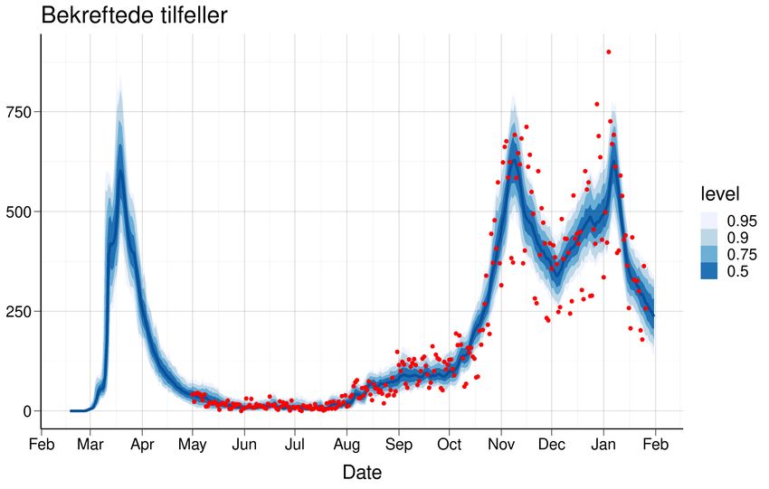
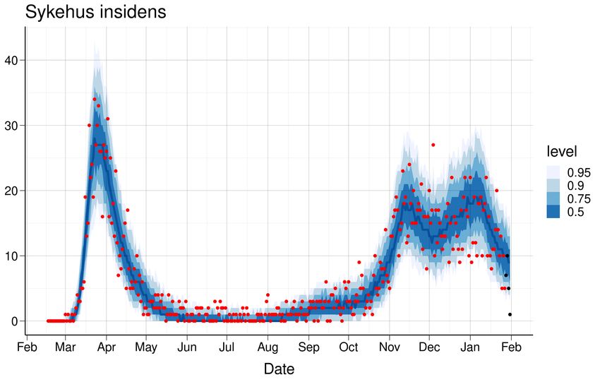
1 Estimated national reproduction numbers
Calibration of our national changepoint model to hospitalisation incidence data and test data leads to
the following estimates provided in table 1. Figure 1 shows the estimated daily number of COVID-19
patients admitted to hospital (1a) and the estimated daily number of laboratory-confirmed SARS-CoV-2
cases (1b), with blue medians and interquantile bands, which are compared to the actual true data,
provided in red. The uncertainty captures the uncertainty in the calibrated parameters in addition to
the stochastic elements of our model and the variability of other model parameters.

 Table 1: Calibration results

 Reff Period
 3.16/3.13(2.41-4.02) From Feb 17 to Mar 14
 0.53/0.53(0.42-0.63) From Mar 15 to Apr 19
 0.65/0.62(0.11-1.08) From Apr 20 to May 10
 0.59/0.59(0.09-1.1) From May 11 to Jun 30
 0.68/0.68(0.08-1.35) From Jul 01 to Jul 31
 1.11/1.1(0.79-1.43) From Aug 01 to Aug 31
 0.94/0.94(0.76-1.15) From Sep 01 to Sep 30
 1.3/1.3(1.08-1.52) From Oct 01 to Oct 25
 1.44/1.44(1.18-1.69) From Oct 26 to Nov 04
 0.83/0.83(0.78-0.88) From Nov 05 to Nov 30
 1.08/1.08(1.04-1.13) From Dec 01 to Jan 03
 0.52/0.51(0.22-0.76) From Jan 04 to Jan 10
 0.77/0.77(0.54-0.97) From Jan 11
 Median/Mean (95% credible intervals)

 (a) Hospital admissions (b) Test data

Figure 1: A comparison of true data (red) and predicted values (blue) for hospital admissions and test data. The last four
data points (black) are assumed to be affected by reporting delay. B) Comparison of our simulated number of positive cases,
with blue median and interquartile bands to the actual true number of positive cases, provided in red. The uncertainty
captures the uncertainty in the calibrated parameters, in addition to the stochastic elements of our model and the variability
of other model parameters. Note that we do not capture all the uncertainty in the test data–our blue bands are quite narrow.
This is likely because we calibrate our model parameters on a 7-days moving average window of test data, instead of daily.
This is done to avoid overfitting to random daily variation. Moving averages over 7 days are less variable than the daily
data.

 3

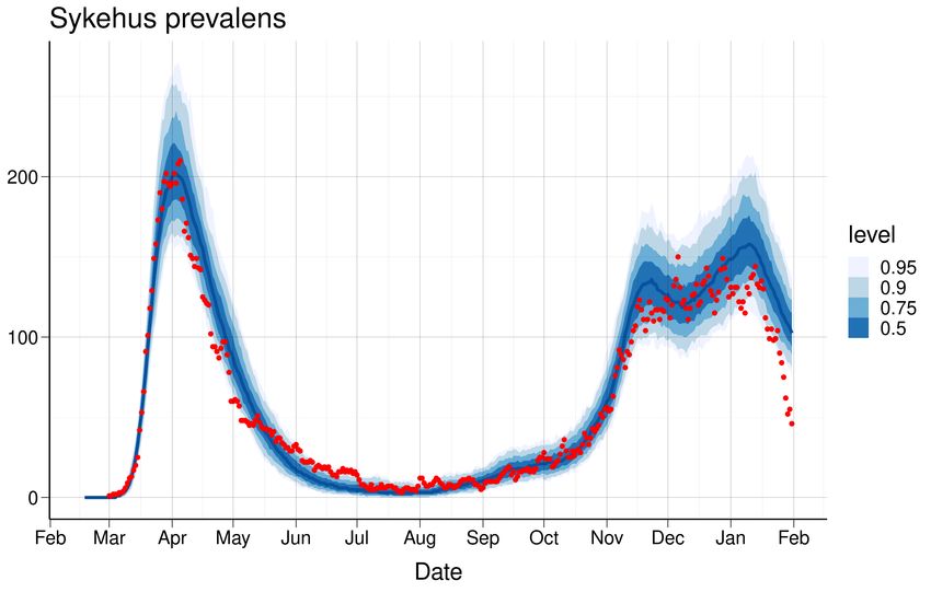
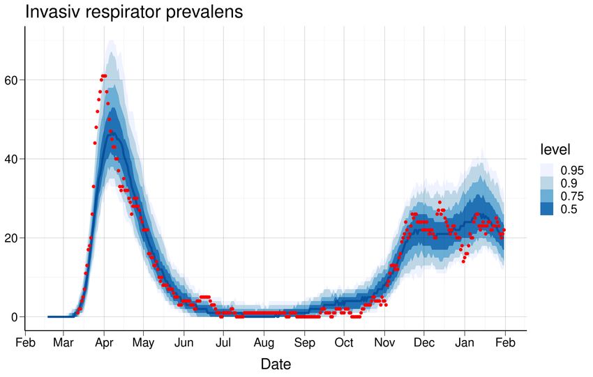
1.1 National SMC-model: Estimated daily reproduction numbers

 In figure 2, we show how our national model fits the national hospital prevalence data (2a) and the
daily number of patients receiving ventilator treatment (2b). Those data sources are not used to estimate
the parameters, and can therefore be seen as a validation of the model assumptions.

 (a) Hospital prevalence (b) Ventilator prevalence

 Figure 2: A comparison of true data (red) and predicted values (blue) for hospital and respirator prevalence.

1.1 National SMC-model: Estimated daily reproduction numbers
In the SMC-model, we allow for estimation of a different reproduction number for each day t. To reduce
spurious fluctuation, we report a 7-days moving average, R(t), representing the average reproduction
number for the whole week before day t. However, until March 8 we keep the reproduction number con-
stant. By assuming a time varying reproduction number R(t), we can detect changes without introducing
explicit changepoints. Thus, we can easier detect unexpected changes.

The SMC model uses the daily number of new admissions to hospital and the daily number of positive
and negative lab-confirmed tests, to estimate all its parameters. Because of the time between infection
and the possibility to be detected as positive by a test, and because if a delay in reporting tests, the data
contain information on the transmissibility until a week before the end of the data (today).

The parameters π0 and π1 related to the probability to detect a positive case by testing are estimated
off-line.

The figure below shows the SMC estimate of the 7-day-average daily reproduction number R(t) from the
start of the epidemic in Norway and until today. In the figure we plot the 95% confidence interval and
quantiles of the estimated posterior distribution of R(t).

 4

1.1 National SMC-model: Estimated daily reproduction numbers

Figure 3: R(t) estimates using a Sequential Monte Carlo approach calibrated to hospitalisation incidence and test data.
The large uncertainty during the last 7 days reflects the lack of available data due to the transmission delay, test delay,
time between symptoms onset and hospitalisation. The green band shows the 95% posterior credibility interval. As we use
test data only from 1 August, the credibility interval becomes more narrow thereafter.

 5

2 National estimate of cumulative (total) number of infections
The national changepoint model estimates the total number of infections and the symptomatic cases that
have occurred (Table 2).
Figure 4a shows the modelled expected daily incidence (blue) and the observed daily number of laboratory-
confirmed cases (red). When simulating the laboratory-confirmed cases, we also model the detection
probability for the infections (both symptomatic, presymptomatic and asymptomatic), Figure 4b. There
are two differences between this estimate of the detection probability and the previous one provided in
figure 4a. In figure 4b, we calibrate our model to the true number of positive cases, instead of using
the test data directly. Furthermore, in figure 4a we use a parametric model to estimate the detection
probability that depends on the true total number of tests performed.

 Table 2: Estimated cumulative number of infections, 2021-01-31

 Region Total No. confirmed Fraction reported Min. fraction
 Norway 114092 (94377; 132619) 62966 55% 47%
 Fraction reported=Number confirmed/number predicted; Minimal fraction reported=number confirmed/upper CI

(a) Number of laboratory-confirmed cases vs model-based esti-(b) Estimated detection probability for an infected case per cal-
mated number of new infected individuals endar day

 Figure 4

 6

3 National 3-week predictions: Prevalence, Incidence, Hospital
 beds and Ventilator beds
The national changepoint model estimates the prevalence and daily incidence of infected individuals
(asymptomatic, presymptomatic and symptomatic) for the next three weeks, aggregated to the whole
of Norway (table 3). In addition, the table shows projected national prevalence of hospitalised patients
(hospital beds) and prevalence of patients receiving ventilator treatment (ventilator beds). The projected
epidemic and healthcare burden are illustrated in figure 5.

 Table 3: Estimated national prevalence, incidence, hospital beds and ventilator beds. Median/Mean (CI)

 1 week prediction (Feb 07) 2 week prediction (Feb 14) 3 week prediction (Feb 21)
 Prevalence 2072/2022 (1031-3420) 1736/1653 (761-3344) 1469/1342 (539-3219)
 Daily incidence 303/289 (136-537) 255/242 (96-535) 218/194 (61-494)
 Hospital beds 93/91 (67-124) 79/79 (50-115) 71/68 (40-111)
 Ventilator beds 17/17 (9-26) 15/14 (7-24) 12/12 (5-22)

Figure 5: National 3 week predictions for incidence (top left), prevalence (bottom left), hospital beds (top right) and
ventilator beds (bottom right)

 7

4 National long-term scenarios: Prevalence, Hospital beds and
 Ventilator beds
Results from 12-month scenario of the calibrated national changepoint model, showing expected preva-
lence (Figure 6a), hospital beds (Figure 6b) and ventilator beds (Figure 6c), in the case where the
transmissibility stays the same as today. The figures are made using the 200 candidate models, where
the reproductive numbers are varying according to their estimated uncertainty as of today. The confi-
dence intervals shown in the plots are two-tailed around the median, and therefore the upper 95% level
shows the 97.5% boundary. Note that age-specific attack rate after 21 days of projection is assumed to
follow the demography in each county, instead of being informed by the current age-distribution of the
laboratory-confirmed cases.

 (a) (b)

 (c)

 Figure 6: Long-term predictions for prevalence (a),hospital beds (b) and ventilator beds (c)

 None of the simulations exceeded a surge capacity of 500 ICU ventilator beds

 8

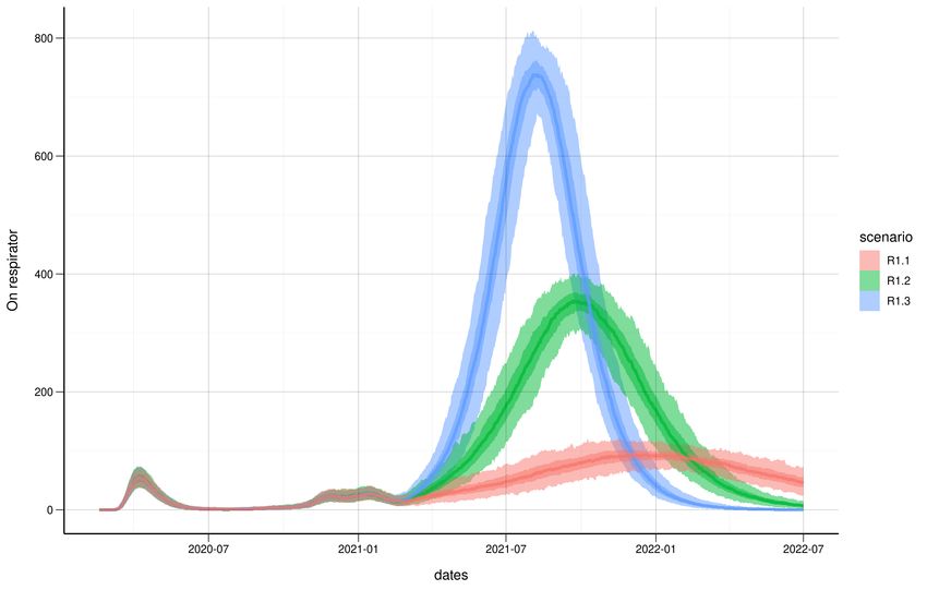
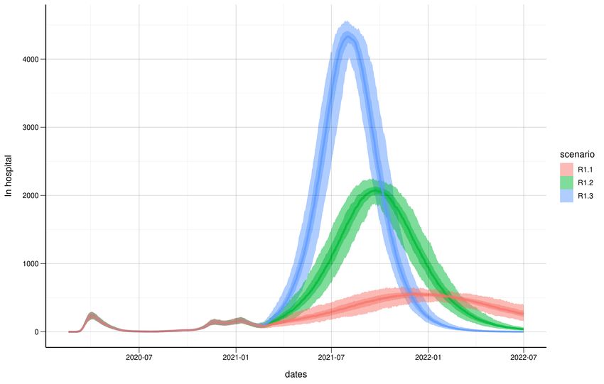
5 National scenario-based long-term predictions: Hospital beds
 and Ventilator beds
NOTE: In this section, we do not include any vaccinations, as planned in the next weeks and months.
The scenarios are therefore not useful anymore. We will soon substitute them with scenarios which
instead include planned vaccinations.

Here we show how the epidemic estimated from the national changepoint model will develop under three
assumed epidemiological scenarios, by fixing the effective reproduction number to be 1.1, 1.2 or 1.3,
from today. We show the daily number of COVID-19 patients in hospital, including patients receiving
ventilator treatment, (Figure 7, and the daily number of patients on ventilator treatment, figure 8.
Note that age-specific attack rate after 21 days of projection is assumed to follow the demography in
each county, instead of being informed by the current age-distribution of the laboratory-confirmed cases.
Additional information about the total attack rate (cumulative incidence) and healthcare burden and
surge capacity for these scenarios are provided in Table 4.

Table 4: Predicted numbers of total infected, total number of hospitalisations, total number needing ventilator treatment,
and the predicted peak number in ward (not in respirator), hospitalised (both with and without ventilator treatment) and
ventilated treatments based on three different scenarios with R effective equal to 1.1, 1.2 and 1.3.

 Reff=1.1 Reff=1.2 Reff=1.3
 Total:
 Attack rate (infected) 785 000(709 000 - 841 000) 1.600.000(1.580.000 - 1.620.000) 2.210.000(2.190.000 - 2.220.000)
 Hospitalisations 24.100(21.600 - 25.700) 49.900(49.000 - 50.600) 69.000(68.300 - 69.800)
 Patients on ventilator 2.330(2.100 - 2.520) 4.790(4.670 - 4.910) 6.620(6.470 - 6.760)
 At peak
 Hospital beds, excl. vent. 507(446 - 565) 1.800(1.700 - 1.890) 3.690(3.570 - 3.820)
 Hospital beds, incl. vent 602(532 - 683) 2.160(2.040 - 2.270) 4.440(4.280 - 4.590)
 Ventilator beds 112(98 - 129) 378(354 - 411) 770(730 - 820)

Figure 7: Predicted number of COVID-19 patients in hospital based on three different scenarios with R effective equal to
1.1, 1.2 and 1.3. Shaded areas show interquartile range and 95% confidence interval around the median.

 9

Figure 8: Predicted number of COVID-19 patients needing ventilator treatment based on three different scenarios with R
effective equal to 1.1, 1.2 and 1.3. Shaded areas show interquartile range and 95% confidence interval around the median.

 10

6 14-day trend analysis of confirmed cases and hospitalisations
 by county
To estimate recent trends in hospitalisation and number of positive tests, we present results in table 5
based on a negative binomial regression where we account for weekend effects. We exclude the last three
days to avoid problems of reporting delay and fit the model using data from 17 days to 3 days before the
current date. We fit a separate trend model for confirmed cases and for hospital incidence. We only fit
a trend model if there has been more than 5 cases or hospitalisations in the 14-day period.

 Table 5: Trend analysis for the last 14 days

 Average daily increase last 14 days Doubling Time (days)
 County Hospitalisations Cases Hospitalisations Cases
 Agder Not enough data 5.2 ( -1.7, 12.8) % Not enough data 13.6 ( -39.3, 5.8)
 Innlandet Not enough data -5.6 ( -14.8, 4.6) % Not enough data -12 ( -4.3, 15.4)
 Møre og Romsdal Not enough data 2.4 ( -6, 11.7) % Not enough data 28.8 ( -11.3, 6.3)
 Nordland Not enough data -2 ( -9.2, 5.8) % Not enough data -34.8 ( -7.2, 12.3)
 Norge -2.9 ( -8.6, 3) % -2.7 ( -4, -1.3) % -23.2 ( -7.7, 23.7) -25.6 ( -16.9, -53)
 Oslo 4 ( -7.2, 16.7) % -2.3 ( -4.4, -0.2) % 17.8 ( -9.3, 4.5) -29.5 ( -15.3, -429.7)
 Rogaland -11.5 ( -28.4, 6) % -15.5 ( -19.2, -11.7) % -5.7 ( -2.1, 11.9) -4.1 ( -3.2, -5.6)
 Troms og Finnmark Not enough data -13.4 ( -22.1, -4.6) % Not enough data -4.8 ( -2.8, -14.7)
 Trøndelag Not enough data -6.8 ( -11.9, -1.5) % Not enough data -9.9 ( -5.5, -46.7)
 Vestfold og Telemark -10.4 ( -24.3, 4.1) % -5.7 ( -9.1, -2.2) % -6.3 ( -2.5, 17.4) -11.8 ( -7.3, -30.9)
 Vestland Not enough data 6.4 ( 1.6, 11.5) % Not enough data 11.2 ( 43.5, 6.4)
 Viken -4.2 ( -11.3, 3.2) % -1.8 ( -3.5, 0) % -16 ( -5.8, 21.8) -38.8 ( -19.3, 8848.1)

 11

7 Mobility data
Number of trips out from each municipality during each day is based on Telenor mobility data. We
observed a large reduction in inter-municipality mobility in March (with minimum reached on Tuesday
17 March), and thereafter we see an increasing trend in the mobility lasting until vacation time in July.
The changes in mobility in July coincides with the three-week ”fellesferie” in Norway, and during August
the mobility resumes approximately the same levels as pre-vacation time. There is however a significant
local variation.
The reference level is set to 100 on March 2nd 2020 for all the figures in this section, and we plot
the seven-day, moving average of the daily mobility. Figure 9 shows an overview of the mobility since
March for the largest municipalities in each county, and Figure 10 shows the total mobility out from all
municipalities in each county, including Oslo. Figure 11 and 12, zooms in on mobility from August 31,
for municipalities and counties, respectively.

Figure 9: Mobility for selected municipalities for all of 2020: Nationally (Norge), Stavanger (1103), Ålesund (1507), Bodø
(1804), Bærum (3024), Ringsaker (3411), Sandefjord (3804), Kristiansand (4204), Bergen (4601), Trondheim (5001), Tromsø
(5401).

 12

Figure 10: Mobility for fylker for all of 2020: Oslo (03), Rogaland (11), Møre og Romsdal (15), Nordland (18), Viken (30),
Innlandet (34), Vestfold og Telemark (38), Agder (42), Vestland (46), Trøndelag (50), Troms og Finmark (54).

 13

Figure 11: Zoom: Mobility from August 31 and onwards: Nationally (Norge), Stavanger (1103), Ålesund (1507), Bodø
(1804), Bærum (3024), Ringsaker (3411), Sandefjord (3804), Kristiansand (4204), Bergen (4601), Trondheim (5001), Tromsø
(5401).

 14

Figure 12: Zoom: Mobility from August 31 and onwards, per fylker: Oslo (03), Rogaland (11), Møre og Romsdal (15),
Nordland (18), Viken (30), Innlandet (34), Vestfold og Telemark (38), Agder (42), Vestland (46), Trøndelag (50), Troms
og Finnmark (54).

 15

2 3 4 5 6
 Norge 66.5 68.1 70.8 69.8 66.0
 Stavanger 57.6 59.6 61.0 65.7 61.0
 Ålesund 72.2 74.5 79.6 82.7 76.2
 Bodø 68.5 72.0 75.7 79.7 83.1
 Bærum 43.1 49.0 50.0 42.2 39.8
 Ringsaker 75.9 72.7 76.4 79.1 73.3
 Sandefjord 56.4 60.4 61.2 61.5 55.5
 Kristiansand 65.0 69.8 71.1 77.8 73.1
 Bergen 63.8 68.4 71.1 74.8 69.3
 Trondheim 57.3 64.5 71.0 75.9 71.9
 Tromsø 72.3 72.8 71.9 73.6 84.8

 Table 6: Municipalities

 2 3 4 5 6
 Oslo 39.7 45.8 47.5 37.4 33.5
 Rogaland 64.6 67.0 68.2 73.3 68.9
 Møre og Romsdal 79.0 79.7 85.8 88.2 81.1
 Nordland 79.9 81.5 84.7 85.6 90.0
 Viken 60.0 63.0 64.4 57.9 53.0
 Innlandet 90.5 82.2 87.6 92.2 85.1
 Vestfold og Telemark 65.0 66.9 68.9 70.4 66.0
 Agder 76.0 78.6 80.6 86.5 87.7
 Vestlandet 74.7 75.6 78.5 81.7 78.5
 Trøndelag 71.3 73.4 79.8 84.1 82.5
 Troms og Finnmark 77.0 77.7 81.0 79.7 85.1

 Table 7: Counties

Weekly mobility for Norway and selected municipalities is displayed in Tables 6 and mobility for counties
is displayed in 7. The percentages in the tables are to be interpreted towards the reference level of
100% for week 10 in March 2020. The color-coding encodes the following: ’Green’ monotonic decrease
in mobility, ’Yellow’ almost monotonic decrease or flat mobility trend, ’Red’ increasing mobility.

 16

7.1 Foreign roamers on Telenor’s network in Norway

7.1 Foreign roamers on Telenor’s network in Norway
An analysis of foreign roamers in Norway from January 2020 has been carried out, to better understand
the potential virus importation. In Figure 13 the total number of roamers per day per county are
displayed. We can see an approximate 40% drop in the number of visiting roamers after the lock-down
in March. The number of visiting roamers recover during the Summer, and there is a spike of visitors in
August followed by a drop again. During October and November the levels of visiting, foreign roamers to
Norway have reached quite high levels, just 10% short of the all-year high for 2020, and Oslo and Viken
have seen big increases in visitors. There is a reduction in visitors during Christmas, and in January
2021 we see an increasing trend again.
 Figure 14 showcases the levels of roamers from the following countries: Poland, Lithuania, Sweden,
Netherlands, Denmark, Latvia, Germany, Spain, Finland and the rest of the world. These levels represent
the total number of foreign, visiting roamers from each of the countries per day in Norway, since October
2020.

Figure 13: The total number of foreign roamers in Norway broken down on different fylker: Oslo (3), Rogaland (11),
Møre og Romsdal (15), Nordland (18), Viken (30), Innlandet (34), Vestfold og Telemark (38), Agder (42), Vestland (46),
Trøndelag (50), Troms og Finmark (54).

 17

7.1 Foreign roamers on Telenor’s network in Norway

Figure 14: National overview of total number of foreign, visiting roamers from Poland, Lithuania, Sweden, Netherlands,
Denmark, Latvia, Germany, Spain, Finland and the rest of the world.

 18

7.2 Foreign roamers per county (fylke) in Norway

7.2 Foreign roamers per county (fylke) in Norway

 19

7.2 Foreign roamers per county (fylke) in Norway

 20

7.3 Mobility analysis of Nordre Follo in connection with the recent cluster of B.1.1.7 cases

 Mean Out Sum Out W02 Sum Out W03 Sum Out W04
 Oslo 2233.7 73407.0 68893.0 38846.0
 Ås 1436.3 42381.0 42980.0 31285.0
 Indre Østfold 473.7 15057.0 14080.0 9922.0
 Nesodden 293.6 8337.0 8378.0 7146.0
 Frogn 238.1 8013.0 6967.0 4272.0
 Vestby 233.2 7868.0 7174.0 4201.0
 Enebakk 175.1 5358.0 4587.0 3054.0
 Bærum 115.1 3802.0 3700.0 1879.0
 Moss 113.9 3744.0 3703.0 2067.0
 Lillestrøm 94.4 3104.0 2856.0 1696.0
 Lørenskog 72.4 2509.0 2257.0 1267.0
 Asker 71.8 2441.0 2137.0 1174.0
 Fredrikstad 65.7 2105.0 2040.0 1312.0
 Sarpsborg 46.6 1588.0 1305.0 989.0
 Ullensaker 40.4 1332.0 1220.0 686.0
 Drammen 22.6 798.0 695.0 380.0
 Våler (Østf.) 17.3 595.0 664.0 296.0
 Nittedal 16.8 587.0 468.0 185.0
 Skiptvet 14.1 446.0 481.0 283.0
 Halden 13.4 474.0 426.0 232.0

 Table 8: Nordre Follo - Outgoing connectivity

7.3 Mobility analysis of Nordre Follo in connection with the recent cluster
 of B.1.1.7 cases
In this Section we will look a bit in detail about the mobility of the municipality Nordre Follo, in light
of the recent cluster of B.1.1.7. We are looking at mobility from three angles: i) The connectivity
pattern of Nordre Follo to other municipalities in Norway, where we both look at outgoing and incoming
connectivity. ii) We analyze the presence of foreign roamers in Nordre Follo, specifically, and finally,
iii) we look at the micro-mobility of the population belonging to Nordre Follo. This is investigated by
looking at the cumulative distributions of maximum distance traveled away from home, and the time
spent away from home.
 We report the total number of movements out of Nordre Follo to other municipalities in Table 8, and
incoming movement in 9. In both cases we show the total number of movements in weeks 2, 3, and 4 of
2021. We also computed the six hour average number of movements since 1.1.2021. The municipalities
are ranked according to the volume of movements. Bærum, that is not bordering with Nordre Follo
has slightly more connections to Nordre Follo than Moss, that is bordering. Otherwise, the other nine
bordering municipalities are the ones with most contacts with Nordre Follo.
 Table 16 below lists the number of movements from the various municipalities into Nordre Follo. The
numbers are very similar, indicating that most of the movements are likely to be for job commuting and
shopping travel.

 21

7.3 Mobility analysis of Nordre Follo in connection with the recent cluster of B.1.1.7 cases

 Mean In Sum In W02 Sum In W03 Sum In W04
 Oslo 2203.2 72111.0 67805.0 37610.0
 Ås 1452.8 43561.0 43315.0 31709.0
 Indre Østfold 475.4 15090.0 14400.0 9951.0
 Nesodden 292.1 8402.0 8192.0 7171.0
 Vestby 251.7 8309.0 7852.0 4486.0
 Frogn 239.5 8084.0 7050.0 4264.0
 Enebakk 178.7 5576.0 4582.0 3225.0
 Bærum 121.6 4009.0 3897.0 1835.0
 Moss 110.8 3573.0 3663.0 2113.0
 Lillestrøm 93.8 3154.0 2874.0 1691.0
 Asker 74.7 2553.0 2276.0 1270.0
 Lørenskog 73.9 2511.0 2264.0 1309.0
 Fredrikstad 63.7 2076.0 1840.0 1331.0
 Sarpsborg 44.1 1464.0 1287.0 885.0
 Ullensaker 37.4 1096.0 1105.0 712.0
 Drammen 23.7 888.0 669.0 452.0
 Nittedal 17.4 623.0 516.0 187.0
 Våler (Østf.) 17.0 553.0 542.0 382.0
 Råde 15.8 578.0 467.0 281.0
 Skiptvet 15.7 452.0 578.0 370.0

 Table 9: Nordre Follo - Incoming connectivity

Figure 17: Number of foreign visitors (roaming on Telenor) present in Nordre Follo since Dec 1st, daily. Left panel: The
trends for Polish and Lithuanian roamers follow the national pattern with a reduction over Christmas and New Year. Right
panel: However, visitors from UK show an increase – near doubling – compared to beginning of December.

 22

7.3 Mobility analysis of Nordre Follo in connection with the recent cluster of B.1.1.7 cases

Figure 18: Here we study mobility within Nordre Follo in January. Micro-mobility in Nordre Follo is measured in two ways:
i) Maximum distance traveled away from home (upper panels), and ii) Time spent away from home (lower panels). We
have compared four different Thursdays (left panels) and five different Fridays (right panels) in January 2021. The most
recent Thursday (violet) and Friday (green) shows a clear left-shift of the cumulative distributions. This left-shift tells that
people in Nordre Follo are now spending less time away from home, and travelling shorter away from home, compared to
the last weeks, as indicated by current local rules.

 23

8 Methods
8.1 Model
We use a metapopulation model to simulate the spread of COVID-19 in Norway in space and time. The
model consists of three layers: the population structure in each municipality, information about how
people move between different municipalities, and local transmission within each municipality. In this
way, the model can simulate the spread of COVID-19 within each municipality, and how the virus is
transported around in Norway.

8.1.1 Transmission model
We use an SEIR (Susceptible-Exposed-Infected-Recovered) model without age structure to simulate the
local transmission within each area. Mixing between individuals within each area is assumed to be ran-
dom. Demographic changes due to births, immigration, emigration and deaths are not considered. The
model distinguishes between asymptomatic and symptomatic infection, and we consider presymptomatic
infectiousness among those who develop symptomatic infection. In total, the model consists of 6 dis-
ease states: Susceptible (S), Exposed, infected, but not infectious (E1 ), Presymptomatic infected (E2 ),
Symptomatic infected (I), Asymptomatic infected (Ia ), and Recovered, either immune or dead (R). A
schematic overview of the model is shown in figure 19.

 Susceptible, S
 / 
 $" " / 
 () ) / 

 Exposed, not
 infectious, no
 symptoms, E1
 , (1 − " ) , "
 Exposed,
 Infectious
 presymptomatic,
 asymptomatic, "
 infectious, E2

 )

 γ
 Infectious,
 symptomatic, I
 γ
 Recovered, R

 Figure 19: Schematic overview of the model.

8.2 Movements between municipalities:
We use 6-hourly mobility matrices from Telenor to capture the movements between municipalities. The
matrices are scaled according to the overall Telenor market share in Norway, estimated to be 48%. Since
week 8, we use the actual daily mobility matrices to simulate the past. In this way, alterations in the
mobility pattern will be incorporated in our model predictions. To predict future movements, we use the

 24

8.3 Healthcare utilisation

latest weekday measured by Telenor, regularised to be balanced in total in- and outgoing flow for each
municipality.

8.3 Healthcare utilisation
Based on the estimated daily incidence data from the model and the population age structure in each
municipality, we calculated the hospitalisation using a weighted average. We correct these probabilities
by a factor which represents the over or under representation of each age group among the lab confirmed
positive cases. The hospitalisation is assumed to be delayed relative to the symptom onset. We calculate
the number of patients admitted to ventilator treatment from the patients in hospital using age-adjusted
probabilities and an assumed delay.

8.4 Seeding
At the start of each simulation, we locate 5.367.580 people in the municipalities of Norway according to
data from SSB per January 1. 2020. All confirmed Norwegian imported cases with information about
residence municipality and test dates are used to seed the model, using the data available until yesterday.
For each case, we add an additional random number of infectious individuals, in the same area and on
the same day, to account for asymptomatic imported cases who were not tested or otherwise missed. We
denote this by the amplification factor.

8.5 Calibration
Estimation of the parameters of the model: the reproduction numbers, the amplification factor for the
imported cases, the parameters of the detection probability and the delay between incidence and test,
is done using Sequential Monte Carlo Approximate Bayesian Computation (SMC-ABC), as described
in Engebretsen et al. (2020): https://royalsocietypublishing.org/doi/10.1098/rsif.2019.0809, where the
algorithm can be found in the supplement.
 The idea behind ABC is to try out different parameter sets, simulate using these, then compare how
much the simulations deviate from the observations in terms of summary statistics. We thus test millions
of combinations of R0 , R1 , R2 , R3 , R4 , R5 , R6 , R7 , R8 , R9 , R10 ,R11 , the amplification factor, and the
parameters for the positive tests, to determine the ones that lead to the best fits to the true number of
hospitalised individuals, from March 10 until the last available data point, and the laboratory-confirmed
COVID-19 cases from May 1 until the latest available data point.
 In the ABC procedure we thus use two summary statistics, one is the distance between the simulated
hospitalisation incidence and the observed incidence, and the other is the distance between the observed
number of laboratory-confirmed cases and the simulated ones. As the two summary statistics are not on
the same scale, we use two separate tolerances in the ABC-procedure, ensuring that we get a good fit to
both data sources.

8.5.1 Calibration to hospitalisation data
In order to calibrate to the hospitalisation data, we need to simulate hospital incidence. The details on
how we simulate hospitalisations are described in Section 8.3, using the parameters provided in Section
9, which are estimated from individual-level Norwegian data, and updated regularly. As our distance
measure, we calculate the squared distance over each time point and each county.

8.5.2 Calibration to test data
We include the laboratory-confirmed cases in the calibration procedure, as these contain additional
information about the transmissibility, and the delay between transmission and testing is shorter than
the delay between transmission and hospitalisation. Therefore, we simulate also the number of detected
positive cases in our model. We assume that the number of detected positive cases can be modelled as a
binomial process of the simulated daily total incidence of symptomatic and asymptomatic cases, with a

 25

8.6 Specifications for the national changepoint model

success probability πt , which changes every day. We also assume a delay d between the day of test and
the day of transmission.
 The data on the number of positive cases are more difficult to use, as the test criteria and capacity
have changed multiple times. We take into account these changes by using the total number of tests
performed on each day, as a good proxy of capacity and testing criteria. Moreover, we choose not to
calibrate to the test data before May 1, because the test criteria and capacity were so different in the
early period. The detection probability is modelled as

 πt = exp (π0 + π1 · kt )/(1 + exp(π0 + π1 · kt )),

where kt is the number of tests actually performed on day t, and π0 and π1 are two parameters that we
estimate, assuming positivity of π1 . We also estimate the delay d. We choose to use a 7-days backwards
moving average for the covariate kt . To calculate the distance between the observed number of positive
tests and the simulated ones we also use a 7-days backwards moving average. We do this to take into
account potential day-of-the-week-effects. For example, it could well be that the testing criteria are
different on weekends and weekdays. However, using instead the number of tests and calibrating on a
daily basis would lead to a larger day-to-day variance. This is likely why we find that the uncertainty
in the simulated positive cases seems somewhat too low, and that we do not capture all the variance
in the daily test data. Moreover, the binomial assumption could be too simple, and a beta-binomial
distribution would allow more variance. A limitation of our current model for the detection probability,
is that we only capture the changes in the test criteria that are captured in the total number of tests
performed.

8.6 Specifications for the national changepoint model
In the national changepoint model, we assume a first reproduction number R0 until March 14, a second
reproduction number R1 until April 19, a third reproduction number R2 until May 10, a fourth repro-
duction number R3 until June 30, R4 until July 31, R5 until August 31, R6 from September 1 until
September 30, R7 from October 1 until October 26, R8 until November 4, R9 from November 5th until
November 30th, R10 from December 1st until December 20th and a twelfth reproduction number R11
from December 21st. This last reproduction number is used for the future. The changepoints follow the
changes in restrictions introduced. In the calibration procedure, we obtain 200 parameter sets that we
use to represent the distributions of parameters.
 After we have obtained the estimated parameters, we run the model with these 200 parameter sets
again, from the beginning until today, plus three weeks into the future (or for an additional year). In
this way, we obtain different trajectories of the future, allowing us to investigate different scenarios, with
corresponding uncertainty.

8.7 Specifications for the regional changepoint model
In the regional changepoint model, each county has its own reproduction numbers, assumed constant in
different periods, just like the national changepoint model. As there are more parameters in the regional
changepoint model, we obtain 1000 parameter sets in the ABC-SMC.
 Calibrating regional reproduction numbers is a more difficult estimation problem than calibrating
national reproduction numbers, as we have a lot more parameters, and in addition less data in each
county. Therefore, we cannot include the same amount of changepoints in the regional model as we can
for the national model. Currently we assume five changepoints (six reproduction numbers) for Viken,
Oslo, Vestland (the three largest counties of Norway), and four changepoints (five reproduction numbers)
in all other counties.
 After we have obtained the estimated parameters, we run the model with these 1000 parameter sets
again, from the beginning until today, plus three weeks into the future (or for an additional year). In
this way, we obtain different trajectories of the future, allowing us to investigate different scenarios, with
corresponding uncertainty.

 26

9 Parameters used today
Figures 20 and 21 indicate which assumptions we make in our model, related to hospitalisation. We
obtained data from the Norwegian Pandemiregister. These estimates will be regularly updated, on the
basis of new data.

 p = 0.85 Ward

 Neg binomial
 Mean = 6.18
 Onset of symptoms Hospital days size = 2.03 Discharged

 back in ward
 Neg. binomial time Neg bi-
 mean 8.87 days Ward ICU Ward
 p = 0.15 nomial, mean
 size = 3.40 13.88 days, size
 Neg. binomial
 Neg. binomial 2.19
 mean 15.89
 mean 1.90 days
 days, size =
 size= 1.37
 2.04

 Figure 20: Hospital assumptions and parameters used before 1 August

 p = 0.905 Ward

 Neg binomial
 Mean = 5.46
 Onset of symptoms Hospital days size = 1.75 Discharged

 back in ward
 Neg. binomial time Neg. bi-
 mean 7.61 days Ward ICU Ward
 p = 0.095 nomial, mean
 size = 3.34 11.79 days, size
 Neg. binomial
 Neg. binomial 1.56
 mean 10.44
 mean 3.22 days
 days, size =
 size = 1.28
 1.24

 Figure 21: Hospital assumptions and parameters used after 1 August

 27

Table 10: Estimated parameters

 Min. 1st Qu. Median Mean 3rd Qu. Max. Period
 R0s 2.286 2.766 3.158 3.129 3.433 4.34 Until March 14
 R1s 0.366 0.496 0.531 0.529 0.567 0.669 From 15 March to 19 April
 R2s 0.003 0.468 0.647 0.622 0.777 1.194 From 20 April to 10 May
 R3s 0.005 0.375 0.585 0.589 0.783 1.368 From 11 May to 30 June
 R4s 0.018 0.403 0.678 0.675 0.912 1.674 From 01 July to 31 July
 R5s 0.553 0.966 1.114 1.099 1.228 1.537 From 01 August to 31 August
 R6s 0.688 0.872 0.936 0.941 1.011 1.283 From 01 September to 30 September
 R7s 0.998 1.217 1.302 1.295 1.377 1.603 From 01 October to 25 October
 R8s 1.097 1.353 1.438 1.441 1.522 1.959 From 26 October to 04 November
 R9s 0.756 0.813 0.829 0.831 0.849 0.904 From 05 November to 30 November
R10s 1.023 1.065 1.08 1.082 1.096 1.149 From 01 December to 03 January
R11s 0.185 0.415 0.516 0.51 0.608 0.829 From 04 January to 10 January
R12s 0.385 0.701 0.773 0.773 0.857 1.032 From 11 January
AMPs 1.007 1.384 1.669 1.698 2.011 2.866 -
 π0 -0.968 -0.135 0.042 0.018 0.216 0.672 -
 π1 5.5e-07 1.8e-05 3.0e-05 3.3e-05 4.3e-05 1.1e-04 -
delays 0 2 3 2.395 3 4 -

 28

30
 Frequency

 Frequency

 Frequency
 50

 25
 20

 10
 10 0

 0

 0
 2.5 3.5 0.35 0.50 0.65 0.0 0.4 0.8 1.2
 R0 R1 R2
 20 40 60

 40
 Frequency

 Frequency

 Frequency
 30
 20

 0 10
 0

 0

 0.0 0.4 0.8 1.2 0.0 0.5 1.0 1.5 0.6 1.0 1.4
 R3 R4 R5

 20 40 60
 10 20 30
 Frequency

 Frequency

 Frequency
 0 10 30

 0

 0

 0.7 0.9 1.1 1.3 1.0 1.2 1.4 1.6 1.2 1.6 2.0
 R6 R7 R8
 20 40 60
 Frequency

 Frequency

 Frequency
 20 40
 10 25
 0

 0

 0

 0.80 0.85 0.90 1.04 1.10 1.16 0.2 0.4 0.6 0.8
 R9 R10 R11
 20 40 60
 Frequency
 0

 0.4 0.6 0.8 1.0
 R12

Figure 22: Estimated densities of the reproduction numbers. National model

 29

Table 11

 R Parameter County From To Pr(R>1)
4.72 (3.59-5.69) R0 Oslo 2020-02-17 2020-03-14 1
3.3 (1.66-4.82) R0 Rogaland 2020-02-17 2020-03-14 1
4.6 (2.62-6.54) R0 Møre og Romsdal 2020-02-17 2020-03-14 1
3.62 (2.18-4.97) R0 Nordland 2020-02-17 2020-03-14 1
3.49 (2.27-4.56) R0 Viken 2020-02-17 2020-03-14 1
3.55 (2.06-4.75) R0 Innlandet 2020-02-17 2020-03-14 1
3.76 (2.44-5.02) R0 Vestfold og Telemark 2020-02-17 2020-03-14 1
3.6 (2.34-4.74) R0 Agder 2020-02-17 2020-03-14 1
3.87 (2.3-5.28) R0 Vestland 2020-02-17 2020-03-14 1
2.78 (0.98-4.43) R0 Trøndelag 2020-02-17 2020-03-14 0.97
2.96 (1.62-4.32) R0 Troms og Finnmark 2020-02-17 2020-03-14 1
0.41 (0.17-0.64) R1 Oslo 2020-03-15 2020-04-19 0
0.72 (0.24-1.21) R2 Oslo 2020-04-20 2020-06-19 0.18
0.54 (0.22-0.89) R3 Oslo 2020-06-20 2020-08-31 0
1.26 (0.74-1.7) R4 Oslo 2020-09-01 2020-09-30 0.85
1.66 (1.47-1.83) R5 Oslo 2020-10-01 2020-11-04 1
1.06 (0.93-1.18) R6 Oslo 2020-11-05 2020-11-30 0.84
1.11 (0.95-1.24) R7 Oslo 2020-12-01 2021-01-03 0.92
0.87 (0.34-1.35) R8 Oslo 2021-01-04 0.31
0.58 (0.16-0.97) R1 Rogaland 2020-03-15 2020-04-19 0.01
0.79 (0.52-1.08) R2 Rogaland 2020-04-20 2020-08-31 0.15
0.86 (0.61-1.09) R3 Rogaland 2020-09-01 2020-11-04 0.12
0.75 (0.35-1.11) R4 Rogaland 2020-11-05 2020-11-30 0.11
0.97 (0.44-1.34) R5 Rogaland 2020-12-01 2021-01-03 0.48
0.87 (0.03-1.97) R6 Rogaland 2021-01-04 0.37
0.75 (0.34-1.13) R1 Møre og Romsdal 2020-03-15 2020-04-19 0.11
0.55 (0.21-0.92) R2 Møre og Romsdal 2020-04-20 2020-08-31 0
0.92 (0.58-1.28) R3 Møre og Romsdal 2020-09-01 2020-11-04 0.28
1.04 (0.61-1.46) R4 Møre og Romsdal 2020-11-05 2020-11-30 0.56
0.52 (0.03-1.1) R5 Møre og Romsdal 2020-12-01 2021-01-03 0.05
0.97 (0.05-2.27) R6 Møre og Romsdal 2021-01-04 0.43
0.46 (0.18-0.76) R1 Nordland 2020-03-15 2020-04-19 0
0.43 (0.13-0.72) R2 Nordland 2020-04-20 2020-08-31 0
0.97 (0.64-1.35) R3 Nordland 2020-09-01 2020-11-04 0.45
0.95 (0.32-1.56) R4 Nordland 2020-11-05 2020-11-30 0.45
0.56 (0.04-1.12) R5 Nordland 2020-12-01 2021-01-03 0.07
1.03 (0.08-2.28) R6 Nordland 2021-01-04 0.49
0.73 (0.55-0.89) R1 Viken 2020-03-15 2020-04-19 0
0.7 (0.45-0.96) R2 Viken 2020-04-20 2020-06-19 0.02
0.87 (0.52-1.18) R3 Viken 2020-06-20 2020-08-31 0.27
1.23 (1.09-1.37) R4 Viken 2020-09-01 2020-11-04 1
0.96 (0.86-1.06) R5 Viken 2020-11-05 2020-11-30 0.2
 0.9 (0.79-1) R6 Viken 2020-12-01 2021-01-03 0.04
0.89 (0.5-1.24) R7 Viken 2021-01-04 0.28
Mean and 95% credible intervals

 30

Table 12

 R Parameter County From To Pr(R>1)
0.48 (0.19-0.77) R1 Innlandet 2020-03-15 2020-04-19 0
0.64 (0.43-0.85) R2 Innlandet 2020-04-20 2020-08-31 0
1.02 (0.74-1.28) R3 Innlandet 2020-09-01 2020-11-04 0.57
0.92 (0.57-1.29) R4 Innlandet 2020-11-05 2020-11-30 0.38
0.47 (0.05-0.92) R5 Innlandet 2020-12-01 2021-01-03 0
0.93 (0.06-2.14) R6 Innlandet 2021-01-04 0.41
 0.3 (0.08-0.52) R1 Vestfold og Telemark 2020-03-15 2020-04-19 0
0.74 (0.45-1.01) R2 Vestfold og Telemark 2020-04-20 2020-08-31 0.03
 0.86 (0.44-1.2) R3 Vestfold og Telemark 2020-09-01 2020-11-04 0.26
0.96 (0.68-1.25) R4 Vestfold og Telemark 2020-11-05 2020-11-30 0.39
 0.69 (0.16-1.1) R5 Vestfold og Telemark 2020-12-01 2021-01-03 0.1
 0.94 (0.1-2.08) R6 Vestfold og Telemark 2021-01-04 0.43
0.66 (0.34-0.97) R1 Agder 2020-03-15 2020-04-19 0.01
 0.4 (0.14-0.7) R2 Agder 2020-04-20 2020-08-31 0
0.64 (0.28-0.99) R3 Agder 2020-09-01 2020-11-04 0.02
 0.82 (0.36-1.3) R4 Agder 2020-11-05 2020-11-30 0.22
0.45 (0.04-0.93) R5 Agder 2020-12-01 2021-01-03 0.01
 1.1 (0.12-2.39) R6 Agder 2021-01-04 0.54
0.44 (0.14-0.76) R1 Vestland 2020-03-15 2020-04-19 0
1.06 (0.83-1.27) R2 Vestland 2020-04-20 2020-08-16 0.63
0.82 (0.28-1.34) R3 Vestland 2020-08-17 2020-09-09 0.28
0.75 (0.29-1.17) R4 Vestland 2020-09-10 2020-11-04 0.12
1.01 (0.67-1.41) R5 Vestland 2020-11-05 2020-11-30 0.5
0.42 (0.03-0.88) R6 Vestland 2020-12-01 2021-01-03 0
1.02 (0.09-2.23) R7 Vestland 2021-01-04 0.5
0.68 (0.28-1.13) R1 Trøndelag 2020-03-15 2020-04-19 0.08
0.78 (0.52-1.02) R2 Trøndelag 2020-04-20 2020-08-31 0.05
 0.7 (0.32-1.03) R3 Trøndelag 2020-09-01 2020-11-04 0.05
0.88 (0.49-1.21) R4 Trøndelag 2020-11-05 2020-11-30 0.29
1.05 (0.62-1.43) R5 Trøndelag 2020-12-01 2021-01-03 0.62
0.73 (0.04-1.71) R6 Trøndelag 2021-01-04 0.27
0.81 (0.43-1.17) R1 Troms og Finnmark 2020-03-15 2020-04-19 0.16
0.67 (0.38-0.93) R2 Troms og Finnmark 2020-04-20 2020-08-31 0
0.81 (0.37-1.22) R3 Troms og Finnmark 2020-09-01 2020-11-04 0.18
1.02 (0.54-1.45) R4 Troms og Finnmark 2020-11-05 2020-11-30 0.53
0.54 (0.06-1.08) R5 Troms og Finnmark 2020-12-01 2021-01-03 0.06
 0.96 (0.08-2.1) R6 Troms og Finnmark 2021-01-04 0.46
1.44 (1.01-2.43) AMP factor All -
Mean and 95% credible intervals

 31

Table 13: Assumptions

 Assumptions Mean Distribution Reference
Mobile Mobility Data
 Telenor coverage 48% https://ekomstatistikken.nkom.no/
 Data updated January 23th
 Data used in the predictions January 22th Fixed Corrected to preserve population
Model parameters
 Exposed period (1/λ1 ) 3 days Exponential Feretti et al 2020
 Pre-symptomatic period (1/λ2 ) 2 days Exponential Feretti et al 2020
 Symptomatic infectious period (1/γ) 5 days Exponential Feretti et al 2020
 Asymptomatic, infectious period (1/γ) 5 days Exponential Feretti et al 2020
 Infectiousness asympt. (rIa ) 0.1 Fixed Feretti et al 2020
 Infectiousness presymp (rE2 ) 1.25 Fixed guided by Feretti et al 2020
 Prob. asymptomatic infection (pa ) 0.4 Feretti et al 2020
Healthcare
 Time sympt. onset to hospitalisation 8.87 days (before August 1st)/ 7.40 (After August 1st) Neg. binomial
 Mizumoto et al 2020
 Fraction asymptomatic infections 40% Fixed
 20% for the old population, Diamond Princess
 % symptomatic and asymptomatic Saljie et al 2020
 infections requiring hospitalization: corrected for: % of elderly living in
 0-9 years 0.1% elderly homes in Norway (last two age groups)
 10 - 19 years 0.1% and corrected for presence among positive tested since May 1.
 20 - 29 years 0.5% Corrected values available in tables ?? and ??
 30 - 39 years 1.1% Fixed
 40 - 49 years 1.4%
 50 - 59 years 2.9%
 60 - 69 years 5.8%
 70 - 79 years 9.3%
 80+ years 22.3%
 % hospitalized patients requiring
 ICU
 Feb - July 15.1% Fixed Estimated from ”Beredskapsregistret BeredtC19”
 August - 8.5%

Probability that an admission has been reported on Monday
 From Sunday 32%
 From Saturday 49% Fixed Estimated from ”Beredskapsregistret BeredtC19”
 From Friday 68%
 From Thursday 86%
 Probability that an admission has been reported
 From one day before 53%
 From two days before 77% Fixed Estimated from ”Beredskapsregistret BeredtC19”
 From three days before 82%
 From four days before 91%
Probability that a positive laboratory test has been reported
 From one day before 6.7%
 From two days before 59% Fixed Estimated from MSIS
 From three days before 90%
 From four days before 97%
Probability that a negative laboratory test has been reported
 From one day before 16%
 From two days before 74% Fixed Estimated from MSIS
 From three days before 92%
 From four days before 98%

 32

Supplementary analysis: EpiEstim estimation of reproduction
number based on laboratory-confirmed cases

To complement the results of the metapopulation model, we present estimates of the temporal evolution
of the reproduction number in Norway based on an analysis of laboratory-confirmed cases. The primary
purpose of this analysis is to provide a more comprehensive perspective on the epidemic situation, taking
into account several data sources.
The hospitalisation data are a less biased information source for the number of infections compared to
case data because the testing criteria in Norway has changed. For this reason, the present results should
be interpreted with caution. During the early part of the period, testing of individuals was mainly based
on travel history to areas with an ongoing outbreak. Since the middle of March, testing is recommended
for people with an acute respiratory infection. From early May, the testing criteria have been expanded
to include less severe symptoms. The analysis of laboratory-confirmed cases does not take into account
the effect of imported cases during the early outbreak in Norway; the early results are less reliable than
later results when the impact of importations is negligible.
EpiEstim method and assumptions: We estimate the instantaneous reproduction number using the
procedure outlined in Thompson et al. (2019). This method, implemented in the EpiEstim R-package,
uses a Bayesian approach to estimate the instantaneous reproduction number smoothed over a sliding
window of 5 days, see figure 23. For the results to be comparable to those of the metapopulation model,
we use the same natural history parameters. We estimate the date of infection for each confirmed case
by first estimating the date of symptom onset and then subtracting 5 days for the incubation period.
We estimate the date of symptom onset from the empirical delay between onset and testing in the
first reported cases. For each case, we draw 100 possible onset dates from the delay distribution; this
gives us 100 epi-curves that we use to estimate the reproduction number. The displayed results are the
combined results from all these 100 simulated epi-curves. The serial interval was assumed to be 5 days
with uncertainty; the serial interval refers to the time between symptom onset between successive cases
in a chain of transmission (see https://www.medrxiv.org/content/10.1101/2020.02.03.20019497v2). To
account for censoring of observations with onset dates in the last few days we correct the observed data
by the mean of a negative binomial distribution with observation probability given by the empirical
cumulative distribution of the onset to reporting date distributions. Due to this correction, the results
from the last few days are uncertain, as indicated by increasing credible intervals.

 5
 Reproduction Number

 4

 3

 2

 1

 Apr Jul Oct Jan
 Date

 Figure 23: Reproduction number estimated using the R package EpiEstim.

 33

FHI COVID-19 modelling team:
 • Birgitte Freiesleben de Blasio - Department of Method Development and Analytics. Norwegian
 Institute of Public Health and Oslo Centre for Biostatistics and Epidemiology, University of Oslo.
 • Francesco Di Ruscio - Department of Method Development and Analytics. Norwegian Institute
 of Public Health.

 • Gunnar Øyvind Isaksson Rø - Department of Method Development and Analytics. Norwegian
 Institute of Public Health.
 • Solveig Engebretsen - Norsk Regnesentral.
 • Arnoldo Frigessi - Oslo Centre for Biostatistics and Epidemiology, University of Oslo and Oslo
 University Hospital.

 • Alfonso Diz-Lois Palomares - Department of Method Development and Analytics. Norwegian
 Institute of Public Health.
 • David Swanson - Oslo Centre for Biostatistics and Epidemiology, Oslo University Hospital.
 • Magnus Nygård Osnes - Department of Method Development and Analytics. Norwegian Insti-
 tute of Public Health.
 • Anja Bråthen Kristoffersen - Department of Method Development and Analytics. Norwegian
 Institute of Public Health.
 • Kenth Engø-Monsen - Telenor Research.

 • Louis Yat Hin Chan - Department of Method Development and Analytics. Norwegian Institute
 of Public Health.
 • Jonas Christoffer Lindstrøm - Department of Method Development and Analytics. Norwegian
 Institute of Public Health.

 • Richard White - Department of Method Development and Analytics. Norwegian Institute of
 Public Health.
 • Gry Marysol Grøneng - Department of Method Development and Analytics. Norwegian Insti-
 tute of Public Health.
 • Chi Zhang - Department of Method Development and Analytics. Norwegian Institute of Public
 Health.

 34