FORECASTING LABOUR PRODUCTIVITY GROWTH IN NORWAY FOR THE PERIOD 2012-2021 USING ARIMA MODELS - Sciendo
←
→
Page content transcription
If your browser does not render page correctly, please read the page content below
FORECASTING LABOUR PRODUCTIVITY GROWTH IN
   NORWAY FOR THE PERIOD 2012-2021 USING ARIMA
                     MODELS

                                   PIROOZ SAMAVATI*

                                  I. INTRODUCTION

        Labour productivity is a relationship between production and the factors
of production (Freeman, 2008). Basically, labour productivity is equal to the ratio
between a volume measure of output (gross domestic product (GDP) or gross
value added) and a measure of input use (total number of hours worked or total
employment) (Freeman, 2008).
More specifically, labour productivity measures the amount of real GDP
produced by an hour of labour. Real GDP grows when aggregate working hours
and labour productivity grow, assuming ceteris paribus. 1
        According to the neoclassical models of growth (such as the Solow
model), labour productivity growth is mainly explained by progress in science
and technology (Kaldor, 1966). This fact helps us to better understand Verdoorn’s
law. Verdoorn’s law states that there is a linear relationship between growth in
output and growth in productivity in the long run (Verdoorn, 1949; Kaldor, 1966).
This relationship can be explained by the theory of cumulative causation.
According to this theory, it is primarily growth in effective demand that
stimulates technological growth through increasing division of labour potential
and through learning-by-doing. The resulting labour productivity increase
stimulates higher outputs through the extension of existing markets and the
opening up of new markets. This suggests that labour productivity gains and
growth in output comprise a mutually reinforcing mechanism (Kaldor, 1966;
Schmookler, 1966; McCombie, 2003; Van Geenhuizen, 2009).2

DOI: 10.2478/wrlae-2013-0048
*
  PhD student working under the supervision of Prof. Jaroslaw Kundera at the Economics
Institute, Faculty of Law, Administration and Economics, Wroclaw University;
pirooz_samavati@yahoo.com
1
  R Freeman, ‘Labour Productivity Indicators’ (2008) OECD Statistics Directorate, Division of
Structural Economic Statistics, 5-15 < http://www.oecd.org/std/labour-stats/41354425.pdf >
accessed 18 November 2013.
2
  N Kaldor, Causes of the Slow Growth in the United Kingdom (Cambridge: Cambridge
University Press 1966) 289; J Schmookler, Invention and economic growth (Harvard University

                                            126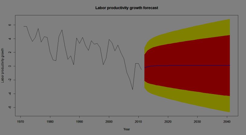
127               Wroclaw Review of Law, Administration & Economics                [Vol 3:1

         To a great extent Norway managed to mitigate the global stagflation of
the 1970s resulting from the global oil crisis through utilizing revenues from oil
exports. Consequently, Norway had higher economic growth and a lower
unemployment rate compared to most of the other Western countries suffering
from the 1970s crisis. However, since Norwegian firms failed to adapt to markets,
Norwegian labour productivity lagged behind the changes in international
markets. This phenomenon, alongside huge growth in oil revenue (from 1973 to
the end of 1985), made a significant contribution to the deindustrialization of
Norway (Grytten, 2008). Thus, compared to the 1948-1970 period, labour
productivity growth in Norway was generally low and variable from the mid-
1970s until the late 1980s (Hagelund, 2009). Figure 1 displays the changes in
annual labour productivity growth in Norway over the last three decades (1971-
2011). As figure 1 suggests, it does not appear that the mean level of labour
productivity growth in the 1990s was higher than the mean rate of growth in the
1970s and 1980s (although possibly the variance of the growth in the 1990s was
lower). Moreover, the level of growth in the 2000s is not greater than the mean
level of growth in the 1990s: it only seems to be greater than the level of growth
in the final two years of the 1990s. There seems to be a change (a fall in the
growth rate) in the middle of the 2000s, before a slight recovery at the end of the
period under consideration (1971-2011). The 2007-2009 financial and economic
crisis in Norway, which resulted from the banking crisis, caused an even greater
fall in labour productivity growth, culminating in it reaching its lowest point in
the previous three decades in 2008. 3 Indeed, a fall in oil revenue and non-oil
sector stagnation resulting from the crisis led to a lower output growth and lower
labour productivity growth (Hagelund, 2009). After 2008 labour productivity

Press,                 Cambridge,                     Massachussets                1966)181-204

accessed 18 November 2013; JP Verdoorn, ‘On the Factors Determining the Growth of Labour
Productivity’ (1949) (in L. Pasinetti (ed.). Italian Economic Papers 59, Vol. II, Oxford: Oxford
University Press 1993) 3-10 ; JSL McCombie , M Pugno, B Soro, ‘Introduction’ (In MP
McCombie, B Soro (eds), Productivity Growth and Economic Performance, Palgrave
Macmillan, London 2002) 1-27; M Van Geenhuizen , DM Trzmielak , DV Gibson, M Urbaniak,
Value-Added Partnering and Innovation in a Changing World (Purdue University Press 2009)
358-362               accessed    18
November 2013; C Kennedy ’Induced bias in innovation and the theory of distribution’ (1964)
in Economic Journal, Vol. 74, 541–547  accessed 18 November 2013; S Scarpetta, T Tressel, ‘Boosting Productivity via
Innovation and Adoption of New Technologies: Any Role for Labour Market Institutions?’(2004)
World         Bank       Policy        Research        Working       Paper,        no.     3273
 accessed 18 November 2013; R Vergeer, A
Kleinknecht, ‘Jobs versus Productivity? The causal link from wages to labour productivity
growth’          (2007)         TU             Delft,       The        Netherlands,          2-6

accessed 18 November 2013.
3
  Similar to Norway, labour productivity growth appeared to fall in some other industrial
European Union (EU) and non-EU countries before the 2007-2009 financial and economic crisis
took place (Appendix A); Therefore, this phenomenon is not specific to Norway. It seems more
general rather than being a consequence of the global financial and economic crisis.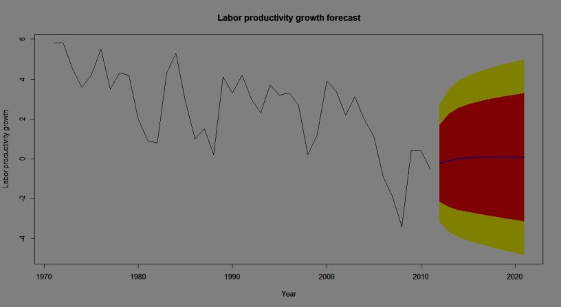
2013]       FORECASTING LABOUR PRODUCTIVITY GROWTH IN                            128
                 NORWAY FOR THE PERIOD 2012-2021 USING ARIMA
                                  MODELS

growth in Norway started to increase. The Norwegian economy also started to
recover in 2010 (IMF, 2012). 4
        Limited access to funds and a decrease in investments as a result of the
financial and economic crisis could lead to a decline in research funding which,
consequently, could slow down technological development and labour
productivity growth in the longer term (Hagelund, 2009). Furthermore, based on
Verdoorn’s law, the reduced output resulting from the economic crisis could
cause a decrease in labour productivity growth. From the perspective of the 2007-
2009 financial and economic crisis in Norway, it is interesting to forecast
Norwegian labour productivity growth for the coming decade. 5

Figure 1. Labour productivity growth time series plot in Norway, 1971-
2011

      Source: Data is extracted from OECD statistics  accessed 18
November 2013.

       Considering the aforementioned facts, this paper focuses on forecasting
labour productivity growth in Norway for the period 2012-2021 through an
autoregressive integrated moving average (ARIMA) model using its successive
values between 1971 and 2011. The Box-Jenkins methodology is applied to
select the appropriate ARIMA model. After identifying the model and
forecasting Norwegian labour productivity growth, this paper discusses the

4
  Ola Grytten, ‘The Economic History of Norway’ (2008) EH.Net Encyclopedia, edited by Robert
Whaples. March 16, 2008  accessed 18
November 2013; K Hagelund, ‘Productivity growth in Norway 1948-2008’ (2009) Special
adviser, Economics Department, Norges Bank, Economic bulletin 2, 4-15  accessed 18 November 2013; IMF Executive
Board Concludes 2011 Article IV Consultation with Norway, Public Information Notice (PIN)
No. 12/9, February 2, 2012  accessed
18 November 2013.
5
  Hagelund (n 4).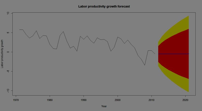
129                Wroclaw Review of Law, Administration & Economics                      [Vol 3:1

selected model. Moreover, it briefly interprets the forecast from an economic
perspective. The paper is organized as follows. Section 2 introduces ARIMA
models. Section 3 presents the Box-Jenkins methodology. In section 4, the model
and the results are obtained. Section 5 discusses the model and the results and
presents a conclusion.

                                     II. ARIMA MODELS

        Since labour productivity growth data has a time-series nature, in order
to model it as a function of its past values a pattern is identified with the
assumption that this pattern will persist in the future. In order to identify patterns
of the series and forecast future points in it, an autoregressive integrated moving
average model (ARIMA) is fitted to the data in this paper.
        Before introducing ARIMA models, it is necessary to briefly present its
two constituents, namely autoregressive models and moving average models
(Hyndman and Athanasopoulos, 2012). In an autoregressive model, the variable
of interest is forecasted using a linear combination of past values of the variable.
Thus, an autoregressive model of order p can be written as: yt=c+φ1yt-1+ φ2yt-
                                                   6
2+…….+ φpyt-p+et, where et is white noise. This is similar to a multiple
regression but lagged values of yt is considered as predictors and c is considered
as an intercept. An autoregressive model is referred to as an AR (P) model. For
an AR (1) model, yt is equivalent to White Noise (WN) when φ1=0. yt is
equivalent to a Random Walk (RW) without drift when φ1=1 and c=0. yt is
equivalent to a Random Walk (RW) with drift when φ1=1 and c0. When φ1 0
and c=0, yt tends to fluctuate between positive and negative values.
Autoregressive models basically apply to stationary data. This being the case, it
is necessary to impose some constraints on the values of the parameters. For
instance, for an AR (1) model: -1
2013] FORECASTING LABOUR PRODUCTIVITY GROWTH IN 130
NORWAY FOR THE PERIOD 2012-2021 USING ARIMA
MODELS
When any MA (q) process can be written as an AR (∞) process, the MA model is
called “invertible”. Invertibility constraints are similar to stationarity constraints.
For example, for an MA (1) model: -1131 Wroclaw Review of Law, Administration & Economics [Vol 3:1
ARIMA models are defined for stationary time series. The Augmented
Dickey–Fuller (ADF) test and the Kwiatkowski–Phillips–Schmidt–Shin (KPSS)
test are two popular tests which evaluate the stationarity of time series. ADF test
tests the null hypothesis of a unit root in a time series sample against the
alternative of stationarity of the time series. The KPSS test tests the null
hypothesis that a time series is level or trend stationary against the alternative
hypothesis that it is a non-stationary unit-root process (Hyndman and
Athanasopoulos, 2012).
Once the model order (the values of p,d, and q) has been indentified, the
parameters including c, φ1,…… φp, θ1,………, θq need to be estimated. A
maximum likelihood estimation (MLE) is used to estimate ARIMA models in R
program. This technique finds the values of the parameters which maximize the
likelihood of obtaining data that have been observed. For ARIMA models, MLE
is very similar to the least squares estimation that would be obtained by
minimizing 2t. In practice, R reports the value of the log likelihood of the data
which is the logarithm of the probability of the observed data coming from the
estimated model. Thus, for given values of p, d and q, R tries to maximize the
log-likelihood of the data when finding parameter estimates (Hyndman and
Athanasopoulos, 2012).
Akaike’s Information Criterion (AIC) is useful to determine the order of
an ARIMA model. It can be written as AIC= -2log (L) + 2(p+q+k+1), where L is
the likelihood of the data, K=1 if c0 and k=0 if c=0. The last term in parentheses
is the number of parameters in the model (including σ2, the variance of the
residuals). For ARIMA models, the corrected AIC can be written as AICc=AIC+
and the Bayesian Information Criterion can be written as BIC=AIC + log (T)
(p+q+k-1), where T is the number of time periods. Better models are obtained by
minimizing either the AIC, AICc, or BIC (Hyndman and Athanasopoulos, 2012).
It is important to note that AICc is recommended to be used as the primary
criterion in selecting the orders of an ARIMA model (Burnham & Anderson,
2004; Brockwell & Davis, 1991).
The point forecast, T+h|T, is defined as the forecast of T+h made at time T. Point
forecasts can be calculated using the following three steps:
1 – Expanding the ARIMA equation so that yt is on the left hand side and all other
terms are on the right.
2 – Rewriting the equation by replacing t by T+h.
3 – Replacing future observations on the right hand side of the equation by their
forecasts, future errors by zero, and past errors by the corresponding residuals.
Beginning with h=1, these steps are then repeated for h=2,3,… until all forecasts
have been calculated (Hyndman and Athanasopoulos, 2012).
ARIMA forecast intervals require far more complex calculations than
point forecasts. The first forecast interval is easily calculated. If is the standard
deviation of the residuals, then a 95% forecast interval is given by T+1|T 1.96
(Hyndman and Athanasopoulos, 2012). The correctness of the forecast intervals
for ARIMA models relies on assumptions that the residuals of a fitted ARIMA
model are uncorrelated and normally distributed (Hyndman and Athanasopoulos,
2012).2013] FORECASTING LABOUR PRODUCTIVITY GROWTH IN 132
NORWAY FOR THE PERIOD 2012-2021 USING ARIMA
MODELS
The forecast intervals from ARIMA models increase as the forecast horizon
increases. The behaviour of the forecast intervals is mainly affected by its
stationarity. For stationary models (with d=0), they initially increase and,
accordingly, they will converge in the long term. For non-stationary models (d
>0), the forecast intervals will continue growing in the long term (Hyndman and
Athanasopoulos, 2012). 9
III. METHODOLOGY
The R programming language (“forecast” package) is used to fit an
ARIMA model to time series data and to do the forecasting. 10 Box-Jenkins
methodology is applied to select the appropriate ARIMA model and forecast the
time series. The Box-Jenkins methodology is capable of identifying the correct
model out of a large class of models through a systematic approach. It employs
both statistical tests for evaluating the model and statistical measures of forecast
uncertainty. This methodology is implemented through the following steps
(Hyndman and Athanasopoulos, 2012):
1. The data is plotted, any unusual observations are identified, and patterns are
evaluated.
2. If it is necessary, the data are transformed using a Box-Cox transformation11
to stabilize the variance and obtain normal distribution.12
3. The stationarity of data is assessed through Augmented Dickey–Fuller (ADF)
and Kwiatkowski–Phillips–Schmidt–Shin (KPSS) tests. If the data are non-
stationary, the first differences of data are taken until data are stationary.
4. The Autocorrelation function (ACF) and partial Autocorrelation function
(PACF) 13 plot of the data (or differenced data) are examined to determine
9
KP Burnham, DR Anderson, Model Selection and Multimodel Inference: A Practical
Information-Theoretic Approach (2nd ed. Springer-Verlag 2002) Chapter 7
accessed 18
November 2013; RJ Hyndman, G Athanasopoulos, Forecasting: principles and practice (An
online textbook, Monash University 2012) Section 8: ARIMA models
accessed 18 November 2013.
10
The R Project for Statistical Computing accessed 18 November
2013.
11
The Box-Cox transformation transforms non-normally distributed data to a set of data that has
approximately normal distribution using BoxCox() function in R. The Box-Cox transformation
is defined as: if λ is not equal to 0, then data(λ)= and if λ is equal to 0, then data(λ)=log(data).
The transformation parameter λ is estimated using automatic selection of Box Cox transformation
parameter (BoxCox.lambda () function in R).
12
GEP Box, DR Cox, ‘An analysis of transformations’ (1964) (B) JRSS 26, 211-246
accessed 18 November 2013.
13
Autocorrelation is the linear dependence of a variable with itself at two points in time. For
stationary processes, autocorrelation between any two observations only depends on the time lag
h between them. Define Cov(yt, yt-h) = γh. Lag-h autocorrelation is given by ρh=Corr(yt,yt-h)=γh/γ0.
The denominator γ0 is the lag 0 covariance that is the unconditional variance of the process.133 Wroclaw Review of Law, Administration & Economics [Vol 3:1
possible candidate models (e.g. to determine whether an AR (p) or MA (q) model
is appropriate).
5. Using information criteria either the AIC, AICc, or BIC, chosen candidate
models are tried to select a better model. Subsequently, a Student’s t-test is used
to test whether the coefficients of the selected model differ significantly from
zero.14 If t-statistics indicates that any of the coefficients of the selected model
fails to differ significantly from zero at the determined significance level (e.g.
α=0.05), that coefficient is set to zero and, consequently, the selected model is
refitted.
6. Goodness of fit for the selected ARIMA model is checked through testing
whether autocorrelation in the residuals is zero, testing the normality and
homoscedasticity (constant variance) of residuals, and testing if the mean of
residuals fluctuates around zero. It should be pointed out that obvious trends
should be removed before normality is checked.
Goodness of fit determines if the residuals look like white noise or not. If
goodness of fit fails and the residuals do not look like white noise, the procedure
resumes from step 4 to find a modified model.
7. Once goodness of fit for the selected model is checked and it is suggested that
the residuals look like white noise, forecasts are calculated.15
IV. THE MODEL AND THE RESULTS
The data is extracted from OECD Statistics.16 Annual growth in GDP per
hour worked (known as labour productivity annual growth rate) in Norway from
1971 to 2011 (figure 1) is the non-seasonal time series to which the ARIMA
model is going to fit. 17 Labour productivity growth time series seems to follow
Correlation between two variables can result from a mutual linear dependence on other variables.
Partial autocorrelation is the autocorrelation between yt and yt-h after removing any linear
dependence on y1, y2, ..., yt-h+1. The partial lag-h autocorrelation is denoted φh,h. The use of these
functions was introduced as part of the Box-Jenkins approach to time series modeling. By plotting
the ACF, the appropriate lags q in MA (q) could be determined. Plotting PACF could help
determine the appropriate lags p in an AR (p) model. Both functions can be used in an extended
ARIMA (p, d, q) model to determine lags q and lags p.
14
The null hypothesis that a coefficient of the selected model is zero is rejected if the absolute
value of t-statistics of that coefficient (the ratio of estimated coefficient to its standard error) is
greater than zα/2 (For larger sample sizes, the t-test procedure gives almost identical p-values as
the Z-test procedure which is based on normal distribution approximation). In this case, a
coefficient of the selected model differs significantly from zero.
15
GEP Box, GM Jenkins, GC Reinsel, Time Series Analysis: Forecasting and Control (3rd ed.
Englewood Cliffs, NJ: Prentice-Hall 1994) 32-33, 66, 68, 70-75, 188, 314-315, 547
accessed 18
November 2013; Hyndman (n 9).
16
Labour productivity growth data in Norway extracted in January 2013 from OECD.Stat accessed 18 November 2013.
17
The data on labour productivity annual growth rate in Norway from 1971 till 2011 is available
in Appendix B.2013] FORECASTING LABOUR PRODUCTIVITY GROWTH IN 134
NORWAY FOR THE PERIOD 2012-2021 USING ARIMA
MODELS
a normal distribution 18 and as figure 1 indicates, it shows no evidence of
changing variance. Consequently, it is not necessary to use a Box-Cox
transformation. In the next step, the stationarity of time series must be tested.
The Norwegian labour productivity growth time series looks non-stationary as
the series has a downward trend and it fluctuates up and down for long periods
(figure 1). Based on the Augmented Dickey-Fuller (ADF) test, the null
hypothesis of a unit root in labour productivity growth time series is failed to
reject at the 5% significance level. In addition, the Kwiatkowski–Phillips–
Schmidt–Shin (KPSS) test indicates that the null hypothesis, that labour
productivity growth time series is level stationary, is rejected in favour of an
alternative hypothesis that it is a non-stationary unit root process at the 5%
significance level. Subsequently, based on the ADF test and KPSS test at the 5%
significance level, the labour productivity growth series is a non-stationary unit
root process. Labour productivity growth series needs to be differenced in order
to be stationary. Based on ADF and KPSS tests, the first difference of the labour
productivity growth series is a stationary process at the 5% significance level
(more details on this can be found in Appendix C).
Therefore, the Norwegian labour productivity growth time series is difference
stationary. It is integrated of order one (I(1)) and it has a unit root.19
After having Norwegian labour productivity growth time series
transformed into a stationary series using the differencing method, an appropriate
ARIMA model is selected.
First of all, the Autocorrelation Function (ACF) and Partial
Autocorrelation Function (PACF) plot for the differenced labour productivity
growth time series are examined. Figure 2 shows the time plot and ACF and
PACF plots (lags 1-20) for the differenced Norwegian labour productivity growth
time series.20
18
The Shapiro-Wilk normality test on labour productivity growth series indicates that the null
hypothesis of normality is failed to reject at 5% significant level (p-value = 0.1557 > 0.05).
19
JD Hamilton, Time Series Analysis (Princeton University Press New Jersey 1994) 514-528
accessed 18 November 2013; A Coghlan, A Little
Book of R For Time Series (Release 0.1. University College Cork, Cork, Ireland 2011) 13-65
accessed 18 November
2013; Hyndman (n 9); DA Dickey, WA Fuller WA, ‘Distribution of the estimators for
autoregressive time series with a unit root’ (1979) Journal of the American Statistical Association
74, 427–431 accessed 18
November 2013; SE Said, DA Dickey, ‘Testing for Unit Roots in Autoregressive-Moving Average
Models of Unknown Order’ (1984) (3) Biometrika 71, 599-607. doi:10.1093/biomet/71.3.599
accessed 18 November 2013; D
Kwiatkowski, PCB Phillips, P Schmidt, Y Shin, ‘Testing the Null Hypothesis of Stationarity
against the Alternative of a Unit Root’ (1992) Journal of Econometrics 54, 159-178
accessed 18 November 2013
20
The values of autocorrelations and partial autocorrelations are presented in Appendix D.135 Wroclaw Review of Law, Administration & Economics [Vol 3:1
Figure 2. Time plot and ACF and PACF plots (lags 1-20) for the differenced
Norwegian labour productivity growth time series
As figure 2 indicates, autocorrelations between lags 1-20 do not exceed
the significant bounds. The ACF looks sinusoidal. Although the partial
autocorrelations between lags 1-20 do not exceed the significant bounds, after
the third lag (which is very close to the lower significance bound), they tail off
to zero. As figure 2 shows, the differenced Norwegian labour productivity growth
time series fluctuates around zero. This fact suggests that the constant term in
ARIMA model is equal to zero. Therefore, an initial candidate model is an
ARIMA (3, 1, 0) without constant.
Candidate models include ARIMA (p, 1, q) models without constant,
where p is between 0 and 3 inclusively, and q varies between 0 and 1 inclusively.
21
The information criteria in Table 2 are used to find a better model.
It is concluded that ARIMA (1, 1, 1) with no constant haa a relative preference
over other models since it has smaller AICc. On the other hand, the auto. arima
() function in the R program22 also identifies ARIMA (1,1,1) with no constant as
an appropriate model.23
Considering equation (2), ARIMA (1, 1, 1) with no constant can be written as
follows:
(1-ar1B)(1-B)yt=(1+ma1B)et
(1-B- ar1B+ ar1B2)yt=(1+ma1B)et
yt - yt-1- ar1yt-1+ar1yt-2=et+ ma1et-1
The final model is: yt= (1+ ar1) yt-1- ar1yt-2+ ma1et-1+ et
Note: ar1 is the first autoregressive coefficient and ma1 is the first moving
average coefficient.
21
PJ Brockwell, RA Davis, Introduction to Time Series and Forecasting (Second edition,
Springer -Verlag, New York 2002) 238-250, 273-320 accessed 18
November 2013; Coghlan (n 19); Hyndman (n 9).
22
The auto.arima() function in R uses a variation of the Hyndman and Khandakar algorithm
which combines unit root tests, minimization of the AICc and MLE to obtain an ARIMA model.
23
Hyndman (n 9).2013] FORECASTING LABOUR PRODUCTIVITY GROWTH IN 136
NORWAY FOR THE PERIOD 2012-2021 USING ARIMA
MODELS
Table 2. Information criteria helping find an appropriate model
Information Criteria
ARIMA Model
sigma^2 Log AIC AICc
likelihood
ARIMA (3, 1, 0) 2.21 -72.8 153.61 154.75
ARIMA (2, 1, 0) 2.411 -74.41 154.83 155.5
ARIMA (1, 1, 0) 2.549 -75.47 154.94 155.27
ARIMA (0, 1, 0) 2.564 -75.59 153.17 153.28
ARIMA (0, 1, 1) 2.531 -75.34 154.69 155.01
ARIMA (1, 1, 1) 2.26 -73.24 152.49 153.16
ARIMA (2, 1, 1) 2.146 -72.27 152.53 153.67
ARIMA (3, 1, 1) 2.091 -71.8 153.59 155.36
The result of ARIMA (1, 1, 1) with no constant for Norwegian labour
productivity growth time series is as follows:
Series: Labourproduc11
ARIMA (1, 1, 1)
ar1 ma1
coefficient 0.5231 -0.8312
standard error 0.2074 0.1328
t-statistics 2.5222 -6.259
p-value 0.0117 < 0.01
sigma^2 estimated as 2.26: log likelihood=-73.24
AIC=152.49 AICc=153.16 BIC=157.56
The final model is: yt= (1.5231) yt-1- (0.5231) yt-2+ (-0.8312) et-1+ et, where yt is
the Norwegian labour productivity growth time series in year t, and et is the white
noise.
The result of ARIMA (1, 1, 1) with no constant model indicates that the
first autoregressive coefficient (ar1) and the first moving average coefficient
(ma1) differ significantly from zero at the 0.05 significance level since the
absolute value of t-statistics (the ratio of estimated coefficient to its standard
error) of the first autoregressive coefficient and the first moving average
coefficient are greater than 1.96 (2.52 and 6.26 respectively)24.
After having the best model selected out of the candidate models and
having the statistical significance of its coefficients tested, its goodness of fit is
checked.
24
P-values from t-statistics are less than 0.05 (0.01 and < 0.01 respectively).137 Wroclaw Review of Law, Administration & Economics [Vol 3:1
In order to check that there is no autocorrelation in residuals, the Ljung-
Box test and the ACF plot of the residuals from the selected model are applied.
The Ljung-Box test is a portmanteau test since it tests the overall randomness
based on a number of lags instead of testing randomness at each distinct lag. The
Ljung-Box test evaluates the null hypothesis that a series of residuals shows no
autocorrelation for a fixed number of lags against the alternative that some
autocorrelation coefficient is non-zero (Box, Jenkins, and Reinsel, 1994; Box and
Pierce, 1970). 25 The Ljung-Box test indicates that the null hypothesis of no
autocorrelation in residuals from ARIMA (1, 1, 1) with no constant for lags 1 -20
is failed to reject at the 0.05 significance level (p-value = 0.8241 > 0.05, and
Q=12.4337 < X20.05, 18=28.87). In addition, the ACF plot of the residuals from the
selected model for lags 1-20 shows all correlations are within the threshold limits
(figure 3). This fact indicates that the residuals are behaving like white noise.
According to its definition, a white noise process is uncorrelated in time. Based
on the Ljung-Box test and ACF plot of the residuals, it is concluded that there is
no evidence for non-zero autocorrelation in residuals of the fitted model at lags
1-20.
Figure 3.The ACF plot of the residuals from ARIMA (1, 1, 1) with no
constant for lags 1-20
In order to check whether the residuals from ARIMA (1, 1, 1) with no
constant have normal distribution, the Shapiro-Wilk normality test of residuals
and normal probability plot of residuals are applied. The Shapiro-Wilk normality
test tests the null hypothesis that the samples come from a normal distribution
against the alternative hypothesis the samples do not come from a normal
25
Box (n 15); GEP Box, DA Pierce, ’Distribution of Residual Autocorrelations in Autoregressive-
Integrated Moving Average Time Series Models’ (1970) Journal of the American Statistical
Association 65, 1509-1526
< http://www.stat.purdue.edu/~mlevins/STAT598K_2012/Box_Pierce_1970.pdf > accessed 18
November 2013.2013] FORECASTING LABOUR PRODUCTIVITY GROWTH IN 138
NORWAY FOR THE PERIOD 2012-2021 USING ARIMA
MODELS
distribution (Shapiro and Wilk, 1965).26 Based on the results of the Shapiro-Wilk
normality test, the null hypothesis of normality of residuals is failed to reject at
the 0.05 significance level (W is large and p-value = 0.1539 > 0.05). The normal
probability plot evaluates whether the data is normally distributed through
plotting the data against a sample from theoretical normal distribution so that the
points should form an approximately straight line. The departure of points from
the straight line suggests departure from normality (Chambers, Cleveland,
Kleiner, and Tukey, 1983).27 The normal probability plot of residuals (figure 4)
indicates that since most of points lie close to a straight line, the data is almost
consistent with a sample from normal distribution. Therefore, based on Shapiro-
Wilk normality test and normal probability plot, it is reasonable to say that the
residuals are approximately normally distributed.
To check whether residuals from ARIMA (1, 1, 1) with no constant have constant
variance, and their mean varies around zero, a time plot of standardized residuals
from this model is used (figure 5). As figure 4.4 indicates, standardized residuals
of the selected model seem to have approximately constant variance over time
(homoscedasticity) although the size of fluctuations at some years is much bigger
compared to others. Furthermore, standardized residuals fluctuate around zero.
The goodness of fit evaluation suggests that the residuals from ARIMA (1, 1, 1)
with no constant look like white noise.28
Figure 4. Normal probability plot of the residuals from ARIMA (1, 1, 1)
with no constant
26
SS Shapiro, MB Wilk, ’An analysis of variance test for normality (complete samples)’ (1965)
(3-4) Biometrika 52, 591-611. doi:10.1093/biomet/52.3-4.591
accessed 18 November 2013.
27
J Chambers, W Cleveland, B Kleiner , P Tukey, Graphical Methods for Data Analysis
(Wadsworth & Brooks/Cole, Pacific Grove, CA 1983) accessed 18 November 2013.
28
In addition to measures mentioned above, in Appendix E, fitted values of labour productivity
growth versus observed values are shown graphically.139 Wroclaw Review of Law, Administration & Economics [Vol 3:1
Figure 5. Time plot of standardized residuals from ARIMA (1, 1, 1) with no
constant
After having goodness of fit checked, using estimated selected ARIMA
model (ARIMA (1, 1, 1) with no constant) labour productivity growth in Norway
for the next 10 years is predicted. In addition, 80% and 95% forecast intervals
for these forecasts are obtained (Table 3).
Table 3. Point forecasts and their 80% and 95% forecast intervals for
labour productivity growth in Norway for the next 10 years using ARIMA
(1, 1, 1) with no constant
Year Point Lo 80 Hi 80 Lo 95 Hi 95
Forecast
2012 -0.2227 -2.1495 1.7040 -3.1695 2.7240
2013 -0.0777 -2.4207 2.2653 -3.6610 3.5056
2014 -0.0018 -2.5583 2.5546 -3.9115 3.9079
2015 0.0379 -2.6594 2.7351 -4.0872 4.1630
2016 0.0586 -2.7478 2.8651 -4.2335 4.3507
2017 0.0695 -2.8305 2.9695 -4.3657 4.5047
2018 0.0752 -2.9099 3.0602 -4.4901 4.6404
2019 0.0781 -2.9868 3.1431 -4.6093 4.7656
2020 0.0797 -3.0618 3.2211 -4.7248 4.8841
2021 0.0805 -3.1349 3.2959 -4.8370 4.9980
Figure 6 displays the observed values of Norwegian time-series labour
productivity growth in the period 1971-2011 (in-sample period) together with
Norwegian time-series labour productivity growth forecasts and their 80% and
95% forecast intervals for the next 10 years (out-of-sample period) using the
selected ARIMA model. The forecasts for the period 2012-2021 are plotted as a
blue line, the 80% forecast interval as an orange shaded area, and the 95%
forecast interval as a yellow shaded area.2013] FORECASTING LABOUR PRODUCTIVITY GROWTH IN 140
NORWAY FOR THE PERIOD 2012-2021 USING ARIMA
MODELS
Figure 6. Observed values of Norwegian time-series labour productivity
growth in the period 1971-2011 (in-sample period) together with its forecast
time-series for the period 2012-2021 (out-of-sample period) using ARIMA
(1, 1, 1) with no constant
As figure 6 shows, Norwegian labour productivity growth time series
continues increasing very slowly and ultimately it goes to a non-zero constant in
the forecast period (2012-2021) following its recovery after 2008.29
DISCUSSION AND CONCLUSION
Norwegian time-series labour productivity growth is difference
stationary. It is integrated of order one (I (1)) and it has a unit root then. Through
Box-Jenkins methodology, ARIMA model is fitted to Norwegian labour
productivity growth time series.
29
Hamilton (n 19) 43-117, 514-528; Brockwell (n 21); C Kleiber , A Zeileis, Applied
Econometrics with R (Springer -Verlag, New York 2008)
accessed 18 November 2013; PSP Cowpertwait, AV Metcalfe, Introductory Time
Series with R (Springer-Verlag, New York 2009)121-128, 137-140
accessed 18 November 2013; Coghlan (n 19); RH Shumway, DS Stoffer, Time Series Analysis
and Its Applications: With R Examples (Springer Texts in Statistics 2010, 3rd ed. 2011) XII,
chapter 3, 83-154
accessed 18 November 2013; Hyndman (n 9); H Akaike, ‘A new look at the statistical model
identification’ (1974) (6) IEEE Transactions on Automatic Control 19, 716-723
accessed 18 November 2013.141 Wroclaw Review of Law, Administration & Economics [Vol 3:1
As AICs (preferred information criterion) indicates, ARIMA (1, 1, 1) with
no constant is selected as an appropriate model among the candidates. The
statistical significance test of coefficients of the selected model indicates that all
coefficients are significant at the 5% level. The auto.arima() function in R also
delivers exactly the same model. If BIC criterion which penalizes the number of
parameters is used, ARIMA (0, 1, 0) with no constant (random walk without a
drift) is obtained as an appropriate model.
From statistical perspective, ARIMA (0, 1, 0) with no constant could be the
second best model since it not only has the smallest BIC, but it has the second
smallest AIC and AICc. In Appendix F, the forecast for time-series labour
productivity growth in Norway for the period 2012-2021 using ARIMA (0, 1, 0)
with no constant (random walk without a drift) is displayed graphically.
However, the random walk model has two obvious weaknesses: 1) The forecasts
for future growth are all negative (It is equal to -0.5), which is not in agreement
with the theory of economic growth through technological advance 2) The
process is not stationary and confidence intervals for the growth rate become
increasingly wide, which is not in accordance with the intuition that over time
the labour productivity growth rate varies within fairly narrow bounds.
Consequently, this random walk model is inappropriate from economic
perspective.
The goodness of fit of the selected model (ARIMA (1, 1, 1) with no
constant) is checked by testing if autocorrelation in its residuals is zero, testing
the normality and homoscedasticity of its residuals, and testing if the mean of
residuals varies around zero. The Ljung-Box test indicates that the null
hypothesis of no autocorrelation in residuals from ARIMA (1, 1, 1) with no
constant for lags 1- 20 is failed to reject at the 5% significance level. The ACF
plot of residuals for lags 1-20 shows that residuals are behaving like white noise.
Therefore, it is concluded that there is no evidence for non-zero autocorrelation
in residuals from the selected model at lags 1-20. The Shapiro-Wilk normality
test of residuals from the selected model (at the 5% significance level) and normal
probability plot of residuals show that it is plausible that the residuals are
approximately normally distributed. The time plot of standardized residuals data
suggests that residuals have approximately constant variance over time. In
addition, standardized residuals fluctuate around zero (indicating that the mean
of residuals varies around zero). As a result, it is concluded that ARIMA (1, 1, 1)
with no constant is well fitted and provides an adequate predictive model for
labour productivity growth, which probably cannot be modified further. In
addition, the assumptions that the 80% and 95% forecast intervals were based on
(that the residuals from the selected model are uncorrelated and normally
distributed) are valid at the 0.05 significance level.
Labour productivity growth is forecasted for the period 2012-2021 using
ARIMA (1, 1, 1) with no constant. The constant c (intercept) has an important
effect on the long-term forecasts obtained from the ARIMA models. If c=0 (zero
intercept) and d=1 (series is non-stationary), the long-term forecasts will go to a
non-zero constant (Hyndman and Athanasopoulos, 2012).2013] FORECASTING LABOUR PRODUCTIVITY GROWTH IN 142
NORWAY FOR THE PERIOD 2012-2021 USING ARIMA
MODELS
By estimating the forecast for labour productivity growth in Norway for the
period 2012-2021 (figure 6) and also for the periods 2012-2031 and 2012-2041
(displayed in
Appendix G) using the selected model (ARIMA (1, 1, 1) with no constant), It is
empirically proven that the long-term forecasts for non-stationary models with
zero intercept will go to a non-zero constant as the forecast horizon increases.
The forecast made using ARIMA (0, 1, 0) with no constant (displayed in
Appendix F) also empirically approves this fact.
For both ARIMA (1, 1, 1) with no constant and ARIMA (0, 1, 0) with no constant,
forecast intervals increase as the forecast horizon increases. As a result, the fact
that for non-stationary models the forecast intervals continue growing in the
long-term is empirically proven.
As discussed before, there seemed to be a change in the Norwegian labour
productivity growth rate (a fall in the growth rate) in the middle of the 2000s,
before a slight recovery at the end of the period under consideration (1971-2011)
occurred. The 2007-2009 financial and economic crisis in Norway (which
resulted from the banking crisis) caused an even greater drop in labour
productivity growth to the extent that in 2008it reached its lowest point in the
previous three decades. After 2008 labour productivity growth started increasing.
Norwegian labour productivity growth continues increasing very slowly and
ultimately it reaches a non-zero constant in the forecast period (2012-2021) and
also over longer periods (2012-2031 and 2012-2041) following its recovery after
2008. A decrease in investment leads to slowed down technological development
in the longer term in a knowledge-based economy like the Norwegian economy,
which is characterised by complex links between service and manufacturing
activities. Therefore, it might initially be concluded that slow technological
development as a result of limited access to funds due to the 2007-2009 financial
and economic crisis in Norway could explain a slowdown in the recovery of
labour productivity growth in the forecast period (2012-2021) and over longer
periods (2012-2031 and 2012-2041). Although the ARIMA (1, 1, 1) with no
constant gives more sensible predictions than random walk without a drift
(ARIMA (0, 1, 0) with no constant), this model also seems to be limited in being
able to describe the data. Firstly, the short-term labour productivity growth rate
is predicted to be less than 0.1%. This seems out of line with the data observed
over the 41-year period as a whole and overly dependent on the data from the
financial and economic crisis period. Also, the 95% confidence interval 2-3 years
(points) after the last observation already covers the range of observations over
the last 41 years, which suggests that picking a number randomly from this range
would be just as good a method as using a time-series model. The reason for this
almost certainly results from the fact that the crisis has changed the underlying
process which the labour productivity growth rate followed in the immediately-
preceding period. Furthermore, the period immediately before the crisis also
covers the technological revolution which can be considered as a contributing
factor to labour productivity growth in Norway. Therefore, it seems unlikely that
a univariate labour productivity growth time series will be rich enough to143 Wroclaw Review of Law, Administration & Economics [Vol 3:1
describe the variation in the data. From the data and the analysis performed, it
seems plausible to conclude that the crisis has changed the underlying process
determining the labour productivity growth rate (at least in the short-term) and
thus, forecasts based on such models are rather unreliable. Finally, it is important
to note that a reliable and effective model which predicts the labour productivity
growth in Norway through employing relevant time series is subject to future
research.
APPENDIX
Appendix A
Labour productivity growth time series plot in some major industrial
countries, 1971-2011
Source: Data is extracted from OECD statistics accessed 18
November 2013.
Appendix B
Labour productivity annual growth rate in Norway from 1971 till 2011:
1971 1972 1973 1974 1975 1976 1977 197 1979 1980 1981 1982
8
5.8 5.8 4.5 3.6 4.2 5.5 3.5 4.3 4.2 2.0 0.9 0.8
1983 1984 1985 1986 1987 1988 1989 1990 1991 1992 1993 1994
4.3 5.3 2.9 1.0 1.5 0.2 4.1 3.3 4.2 3.0 2.3 3.07
1995 1996 1997 1998 1999 2000 2001 2002 2003 2004 2005 2006
3.2 3.3 2.7 0.2 1.2 3.9 3.4 2.2 3.1 2.0 1.1 -0.9
2007 2008 2009 2010 2011
-1.9 -3.4 0.4 0.4 -0.52013] FORECASTING LABOUR PRODUCTIVITY GROWTH IN 144
NORWAY FOR THE PERIOD 2012-2021 USING ARIMA
MODELS
Appendix C
The result of the Augmented Dickey Fuller test (ADF) for labour
productivity growth time series:
Augmented Dickey-Fuller Test
data: Labourproduc11
Dickey-Fuller = -2.5419, Lag order = 3, p-value = 0.3604
alternative hypothesis: stationary
Conclusion: The p-value of the ADF test (0.3604) is greater than 0.05. Therefore,
the null hypothesis of a unit root in labour productivity growth time series is
failed to reject against the alternative that the series is stationary at the 5%
significance level.
The result of the KPSS test for labour productivity growth time series:
KPSS Test for level stationarity
data: Labourproduc11
KPSS Level = 1.0548, Truncation lag parameter = 1, p-value = 0.01
Warning message:
In kpss.test(Labourproduc11, null = "Level") :
p-value smaller than printed p-value
Conclusion: The p-value of the KPSS test is smaller than 0.05. Therefore, the
null hypothesis that labour productivity growth time series is level stationary is
rejected in favour of alternative hypothesis that it is a non-stationary unit-root
process at the 5% significance level.
The result of the Augmented Dickey Fuller test (ADF) for the differenced
labour productivity growth time series:
Augmented Dickey-Fuller Test
data: diff(Labourproduc11)
Dickey-Fuller = -5.0319, Lag order = 3, p-value = 0.01
alternative hypothesis: stationary
Warning message:
In adf.test(diff(Labourproduc11)) : p-value smaller than printed p-value
Conclusion: The p-value of the ADF test is smaller than 0.05. Therefore, the null
hypothesis of a unit root in the differenced labour productivity growth time series
is rejected in favour of the alternative that the series is stationary at the 5%
significance level.
The result of the KPSS test for the differenced labour productivity growth
time series:
KPSS Test for level stationarity
data: diff(Labourproduc11)
KPSS Level = 0.0291, Truncation lag parameter = 1, p-value = 0.1
Warning message:145 Wroclaw Review of Law, Administration & Economics [Vol 3:1
In kpss.test(diff(Labourproduc11)) : p-value greater than printed p-value
Conclusion: The p-value of the KPSS test is greater than 0.05. Then, the null
hypothesis that the differenced labour productivity growth time series is level
stationary is failed to reject against the alternative hypothesis that it is a
nonstationary unit-root process at the 5% significance level.
Appendix D
Autocorrelations for the differenced labour productivity growth time series
by lag
0 1 2 3 4 5 6 7 8 9 10
1.000 -0.086 -0.231 -0.223 -0.103 0.070 0.152 -0.014 0.002 -0.070 0.015
11 12 13 14 15 16 17 18 19 20
0.066 -0.049 0.114 -0.112 -0.112 0.060 -0.039 0.062 -0.100 0.160
Partial Autocorrelations for the differenced labour productivity growth
time series by lag
1 2 3 4 5 6 7 8 9 10 11
-0.086 -0.240 -0.287 -0.268 -0.168 -0.054 -0.133 -0.040 -0.086 -0.010 0.044
12 13 14 15 16 17 18 19 20
-0.051 0.169 -0.046 -0.076 0.014 -0.146 -0.053 -0.290 0.08
Appendix E
Observed values of Norwegian labour productivity growth time series
between 1971-2011 versus its fitted values in the same period using the
selected ARIMA model (ARIMA (1, 1, 1) with no constant)2013] FORECASTING LABOUR PRODUCTIVITY GROWTH IN 146
NORWAY FOR THE PERIOD 2012-2021 USING ARIMA
MODELS
Appendix F
The forecast for labour productivity growth time series in Norway for the
period 2012-2021 using ARIMA (0, 1, 0) with no constant
Note: The forecasts for the period 2012-2021 are plotted as a blue line, the 80%
forecast interval as an orange shaded area, and the 95% forecast interval as a yellow shaded
area.
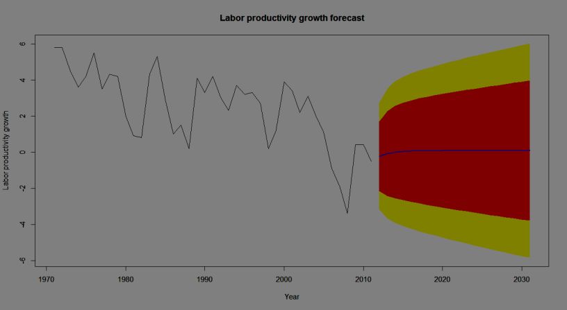
Appendix G
a) A 20-year forecast (2012-2031) for Norwegian labour productivity
growth time series using the selected ARIMA model (ARIMA (1, 1, 1) with
no constant)
Note: The forecasts for the period 2012-2031 are plotted as a blue line, the 80%
forecast interval as an orange shaded area, and the 95% forecast interval as a yellow shaded
area.
b) A 30-year forecast (2012-2041) for Norwegian labour productivity
growth time series using the selected ARIMA model (ARIMA (1, 1, 1) with
no constant)147 Wroclaw Review of Law, Administration & Economics [Vol 3:1
Note: The forecasts for the period 2012-2041 are plotted as a blue line, the 80%
forecast interval as an orange shaded area, and the 95% forecast interval as a yellow shaded
area.You can also read