Journal of Economics Library - KSP Journals

Journal of Economics Library
 www.kspjournals.org
Volume 7 September 2020 Issue 3

 The impact of increasing VAT rate on state
 revenue, a South African case

 By Cathrine Thato KOLOANE a†
 & Mangalani Peter MAKANANISAab

Abstract. The study seeks to evaluate the impact of the increase in VAT rate from 14% to
15% on the state revenue as well as on future VAT collections. VAT historical data spanning
from April 2009 to March 2018 (108 observations) on a fixed rate of 14% was obtained.
Assuming no change on the 14% VAT rate, (0,1,1)(0,1,1)12 was fitted to the data to
predict the collection of R311.2bn and R326.7bn for 2018/19 and 2019/20 respectively. The
difference between prediction (at 14% rate) and actual realisation of R324.8bn and R346.7bn
for the same period (at 15%rate) was computed to get the impact. Based on the model fitted
values, a percentage increase in VAT rate increased payments by 4.2%in 2018/19 and 5.8%in
2019/20.This results in a slight increase in the total state revenue of 1.1% and 1.5% in 2018/19
and 2019/20 respectively. Furthermore, the model forecast R313.9bn to be collected in
2020/21 at 15% rate, the lower collection is due to the covid-19 impact on revenue collection.
The usage of these types of models will assist the South African government in their
budgetary plans and future decisions by taking into account more accurate projected VAT
collection. However, monitoring of the model is crucial as the prediction power deteriorate
in the long run.
Keywords. South African Revenue Service (SARS), Value Added tax (VAT) and Seasonal
Autoregressive Integrated Moving Averages (SARIMA).
JEL. H24, C15, E37.

 1. Introduction

V
 alue added tax (VAT) is an indirect tax which is levied on
 consumption of goods or services. It is the second largest tax,
 having a fixed tax rate of 14% (Tax Statistics, 2019). Since 1993, the
VAT rate had remained fixed at 14%, lower compared to other countries.
The former minister of finance, Mr Malusi Gigaba, during parliamentary
budget speech on the 21 February 2018 revised the VAT rate upwards by
1% to 15% and declared it to be effective from 01 April 2018 onwards as one
of the tax proposals designed to generate more tax revenue for the SARS
fiscal year 2018/19. However, basic foods such as brown bread, dried beans,
maize meal, and rice will remain zero rated to limit the impact on the
vulnerable and poorest household (Budget Speech, 2018).
 It is widely known that the collection of the state revenue is related to
the economic performance of Gross Domestic Product (GDP) or some

aa†South African Revenue Service, Operational Research, Pretoria, South Africa.
 . +2782 906 0090 . tkoloane09@gmail.com
b South African Revenue Service, Operational Research, Pretoria, South Africa.

 . +2782 456 4669 . manginduvho@gmail.com

Journal of Economics Library
components of GDP, which is normally referred to as the base. The VAT
base would be total household consumption. The increase in VAT is good
for the state to function at its maximum capacity and the consumers may
have some relief from the zero rated goods and services. However, the
burden of a percentage increase in VAT will heavily affect poor citizens.
 VAT contributes 25% to total tax revenue and6.6% to the South African
nominal GDP. During fiscal year 2018/19 the registered VAT vendors were
802 957 from which 448 710 (55.9%) were active. The vendors were
distributed into companies and close corporations (77.2%), Individuals
(17.3%), Trust (2.8%), Partnerships (1.7%) and others (1%) (Tax Statistics,
2019).
 The VAT payments by sector for the fiscal year 2018/19 shows that
finance was the highest, contributing 158.9 billion (42.1%), followed by
wholesale at R55.8 billion (14.8%), manufacturing at R53.8 billion (14.2%),
communication, social & personal service at R24.0 billion (6.4%),
construction at R22.4 billion (5.9%), transport, storage & communication at
R22.4 billion (5.9%), mining & quarrying at R14.0 billion (3.7%) and other
sectors share the remaining R224 billion (7.0%)(Tax Statistics, 2019).
 The biggest debatable scenarios for the economists, statisticians and
econometricians analysing the South African economic outlook just before
the beginning of fiscal year 2018/19, was that if VAT is increased by 1% in
2018/19 fiscal year (first increase since 1993):
  What would be the impact of this increase to the economy and how
would this affect the collection of VAT? Will this affect the economy
positively or negatively?
  How can we measure the impact of this change? and
  How much can be expected from the economy beyond 2017/18
fiscal year?
 This study aims to evaluate the impact of the 1% increase in the VAT
rate starting from fiscal year 2018/19 by predicting VAT collections for
2018/19 and 2019/20 using the historical data at 14% rate and compare
predictions with the actual realisation of VAT at 15% rate for the same
period. The prediction utilises the commonly used time series model,
SARIMA.
 This paper is organised as follows; section 2 presents the literature
review, section 3 is the theoretical models, section4 shows the empirical
results and analysis, and section 5 discusses model results and limitations.
Conclusions and recommendations are provided in sections 6.

 2. Literature review
 Prediction or forecasting plays an integral part on planning and
decision-making. Lack of planning might result in failure for the
organisation. Different types of methods exist to predict or forecast the
continuation of a historical trend. These methods could be classified either
as qualitative or quantitative and the applications of these methods have
their own advantages and disadvantages.
 C.T. Koloane & M.P. Makananisa, 7(3), 2020, p.123-136.
 124

 124

Journal of Economics Library
 Under the quantitative methods, sufficient quantitative information
should be available to build a model, which relates one variable, referred to
as a response variable, to one or more explanatory variables. Such
forecasting techniques are referred to as regression methods. The other
quantitative technique is a time series model, which relates current or
future occurrence to the historical patterns of the same variable. However,
qualitative methods are used when there is little to no quantitative
information, but sufficient qualitative information exists (Hyndman et al.,
1998).
 Various literature around the globe support the use of time series
models to predict tax revenue. Edzie-Dadzie (2013) used time series
analysis to forecast Ghana’s VAT revenue. The aim of the paper was to
study the behaviour pattern and trend in Ghana’s VAT revenue and to
choose the best model based on high predictability level among various
ARIMA models. Yearly import and domestic VAT observations covering
the period 1999 to 2009 (132 observations) were examined. The data was
secondary data collected from the Research, Monitoring and Planning
Department of the VAT Service and Monitoring and Evaluation Unit of
CEPS, Headquarters Accra. Time series analysis was used to model the
VAT historical patterns. An ARIMA (2, 1, 2) was found to be the best model
to forecast domestic VAT revenue and an ARIMA (2, 1, 1) was found to be
the best model to forecast import VAT revenue. A forecast of future VAT
revenue for the next thirty-six months was done.
 In their study on VAT revenue modelling, Gumbo & Dhliwayo (2018)
used three different methodologies to forecast VAT revenues. The authors
tested Exponential Smoothing, Elasticity Approach and the Effective tax
rate approach to forecast VAT revenues. Secondary annual data used for
this study covered the period 2010 to 2013 and was collected from the
government of Zimbabwe publications, the International Monetary Fund
(IMF), the World Bank, RBZ, Zimbabwe Revenue Authority (ZIMRA) and
ZIMSTAT.VAT revenue data for the year 2009 was not available from
ZIMRA. Exponential Smoothing had the lowest relative absolute forecast
errors for the years 2012 and 2013compared to the other forecasting
techniques. The study recommends the adoption of a systematic VAT
revenue forecasting approach and the insulation of the revenue forecasting
process from political interference.
 Similarly, Okseniuk (2015) conducted a study to show the use of moving
averages, correlation and regression analysis in order to forecast VAT
revenue. In addition, the author analysed the efficiency of the methods,
computed a forecast for the years 2014–2016 and identified key reasons of
the problems of VAT forecasting. The sample covering the period 2007 to
2013 was collected from the official websites of the Ministry of Finance and
Treasury. The method of correlation and regression analysis was found to
provide more precise forecasts compared to the moving average method.
However, both methods do not take into account the change in tax rates
and the introduction of differentiated rates. This is necessary in order to
 C.T. Koloane & M.P. Makananisa, 7(3), 2020, p.123-136.
 125

 125

Journal of Economics Library
improve the moving average method and the method of correlation and
regression.
 In another related study, “Forecasting tax revenues using time series
techniques – a case of Pakistan”, Streimikiene et al., (2018) collected 31 years
of data from July 1985 to December 2016 to forecast tax revenue of Pakistan
for 2017. The authors used three different time series techniques, namely
AR model with seasonal dummies, ARIMA model and the Vector
Autoregression (VAR) model and evaluated the efficiency of the model by
using Root Mean Squared Error (RMSE) test. The data was collected from
the different issues of the Pakistan Bureau of Statistics (PBS) monthly
bulletin. The study indicated that the ARIMA model forecasted the best
values of total tax revenue because the value of the RMSE was minimum
compared to the AR model with seasonal dummies and the VAR model.
 In the case of Ukraine, Legeida & Sologoub (2003) developed an ARIMA
model to forecast VAT revenue in the short run. The aim of the paper was
to test different methodologies for forecasting VAT revenues. The primary
source of data was budget execution reports released by the State Treasury
of Ukraine (VAT revenue plan and execution) and reports of State Tax
Administration (VAT exemptions). Furthermore, the data from the State
Statistics Committee (on GDP) and the data of the National Bank of
Ukraine (on exports and imports) for VAT base calculation was collected.
The data from the input-output tables was used to estimate the effective
VAT rate. To build an econometric model, the readily available data for
1998-2002 (on a monthly basis) was used. The ARMA (2, 6) model provided
a reasonable forecast of VAT revenues for 2003 that was fully consistent
with government projections for the 2003 budget. The results revealed that
actual VAT revenues are less than a half of potential VAT revenues.
 Furthermore, Ofori (2018), in his paper titled “VAT revenue forecasting
in Ghana”, estimated VAT revenue by using a sample of monthly
observations spanning from 2002 to 2017. The ARIMA with intervention
analysis method of forecasting outperformed the Holt trend model in
forecast accuracy and precision. The ARIMA model was then used to
forecast monthly VAT revenues for the next 24 months. The paper
recommends that the ARIMA with intervention analysis model should be
compared with the in-house model used at Ghana Revenue Authority for
forecast accuracy and prediction and if it out performs the in-house model,
it should be adopted by the Ghana Revenue Authority in forecasting
monthly VAT revenues for the purpose of government budgets.
 In another related study, Nandi et al., (2014) conducted a study to
identify an appropriate model to forecast tax revenue. The models under
study were ARIMA SARIMA multiplicative approach, Holt-Winters
seasonal multiplicative approach and the Holt-Winters seasonal additive
approach. The sample of monthly tax revenue spanning from July 2004 to
November 2012 (101 observations) was collected from the Bangladesh
Ministry of Finance. Out of the 101observations, 84 data points were used
to specify a model and the remainder was used to check for the fit of the
 C.T. Koloane & M.P. Makananisa, 7(3), 2020, p.123-136.
 126

 126

Journal of Economics Library
specified model. The results revealed that the Holt-Winter seasonal
multiplicative approach was the most appropriate method with minimum
forecast error.
 In the case of South African literature, Erero (2015) used the dynamic
computable general equilibrium (CGE) model to analyse the effect of
increases in VAT (by 1% to 5%) to other sectors and the national income
(GDP), using annual data for the period 2012 to 2018. The findings showed
that an increase of 1% in VAT rate will not affect lower income household
but will impact the investments through the price of capital. Hence the
GDP will increase slightly by around 0.022% in 2013 to 0.114% in 2008 and
also show positive impact for the period 2013 to 2018. However, this study
uses shorter time series and does not show how the VAT will increase for
the period 2018/19 and beyond in monetary terms or percentage change (or
growth) from 2017/18 financial year.
 The availability of historical quantitative data for the South African VAT
payments allows this study to focus on the time series quantitative
methods, SARIMA model, to predict and answer the question; what is the
impact of the increased VAT rate for 2018/19 and beyond?

 3. Theoretical models
 3.1. ARIMA/SARIMA model
 The autoregressive integrated moving averages (ARIMA) model or the
Box-Jenkins methodology relates the current observation to its historical
occurrence and builds the relationship and stochastic error term, referred to
as model fitting (Gujarati, 2003). This means that the series to be forecast is
generated by a random process with a structure that can be described. The
description is given in terms of the randomness of the process rather than
the cause and effect used in regression models (Pindyck & Rubinfeld, 1998).
This type of model requires the data to be stationary around the mean and
the variance.
 As stated by Gujarati & Porter (2009), in practice most time series are
non-stationary. Normal ARIMA models are not applicable to such data.
This implies that the series should be differenced to obtain stationarity as
follows: ∇ = − −1 = (1 − ) . The series may become stationary
when d = 1 or d = 2 in practice. When this is done, the resultant series is
ARIMA (p, d, q).
 The ARIMA (p, d, q) is expressed as a back-shift operator in equation 1,
alternatively, as the more general model in equation 2.

 1 − 1 B − 2 B 2 − ⋯ − B 1 − B = 0 + 1 − 1 B − 2 B 2 − B 
 (1)
 1 B 1 − B = (B) (2)

 where B = 1 − 1 B − 2 B 2 − ⋯ − B , B = 1 − 1 B − 2 B 2 −
⋯ − B , 1 − B = , d is the degree of differencing and is a series

 C.T. Koloane & M.P. Makananisa, 7(3), 2020, p.123-136.
 127

 127

Journal of Economics Library
 of random errors each with zero mean and constant variance 2 . The model
 in equation 1 for the series is referred to as the autoregressive integrated
 moving average model of order (p,d,q), and is denoted by ARIMA(p,d,q).
 Note that the AR(p), MA(q) and ARMA(p, q) models are special ARIMA (p,
 d, q) models. For example, the ARMA(p, q) model is the ARIMA(p,0,q)
 model, the AR(p) model is the ARIMA(p,0,0) model and the MA(q) model
 is the ARIMA(0,0,q) model.
 Time series data can be non-stationary, and/or, exhibit the rise and fall
 on the fixed points for an observed period. Such series are called seasonal
 time series data and can be seasonally differenced to obtain stationarity.
 The general seasonal autoregressive integrated moving average (SARIMA)
 model is represented by ARIMA(p,d,q) (P,D,Q)s, using a back-shift
 operator. It is then expressed as:

 B Φ B = + B Θ(B ) (3)

 where = 1 − B 1 − B s D = 1 − B d − B sD + B sD +d is the
 product of seasonal differencing D and non-seasonal differencing d, s is the
 series seasonality which takes the value 4 for quarterly time series data and
 12 for monthly time series data, is the constant term and is the
 disturbance or error term at time t.
 Furthermore Yurekli, Kurunc & Ozturk (2005), and Maindonald &
 Braun (2003) express ϕ B , Φ B s , θ B and Θ(B s ) as follows;

 B = 1 − 1 B − 2 B 2 − ⋯ − B is non-seasonal AR components of order p.
 Φ B = 1 − Φ1 B − Φ2 B 2 − ⋯ − Φ B P is seasonal AR components of order P.
 B = 1 − 1 B − 2 B 2 − ⋯ − B is the non-seasonal MA components of order q
Θ B = 1 − Θ1 B S − Θ2 B 2s − ⋯ − Θ B Qs the seasonal MA components of order Q.

 Typical methods of estimating the model parameters are either the least
 squares method and/or the maximum likelihood methods. These methods
 are briefly reviewed under the assumption that the identified tentative
 ARIMA and SARIMA models for a given time series model in equation 2
 and 3 above can be re-rewritten for error term (assuming that = 0)as
 equation 4 and 5, respectively:

 = B 1 − B −1 (B) (4)
 = B −1 (B)Φ(B s ) Θ−1 (B s ) (5)

 3.2. In-sample measures
 Given time series where t = 1, 2,…, T, there may be several competing
 ARIMA/SARIMA models for forecasting. According to Wei (2006), the
 models can be compared for goodness of fit using Mean Percentage Error
 (MPE), Mean Square Error (MSE), Mean Absolute Error (MAE) or Mean
 Absolute Percentage Error (MAPE), Akaike's Information Criterion (AIC)
 and the Bayesian Information Criterion (BIC), depending on the
 C.T. Koloane & M.P. Makananisa, 7(3), 2020, p.123-136.
 128

 128

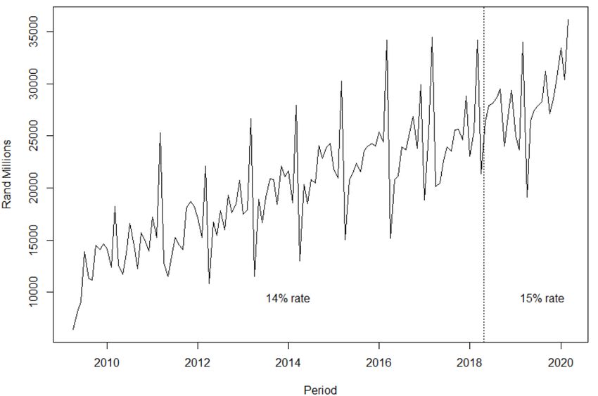
Journal of Economics Library
criterion/criteria which one chooses to use. The smaller the value of the
statistic the better.
 The crucial part in ARIMA/SARIMA models is to examine the model
residual to identify if they are distributed normally around zero over the
time period given. Here the graphical visualisation such as residual
histogram and qq-plot could be of assistance. However, the most
commonly used statistic to assess if the residuals are white noise process is
the Ljung-Box Statistics which test for autocorrelation at lag k to see if the
residuals are approaching zero and it is also a 2 distribution with m
degrees of freedom for larger sample size n. This statistic can be
mathematically represented as follows:

 2
 = ( + 2) =1 − (6)

 where 2 is the squared autocorrelation at lag k for the selection of the
 
model autoregressive and moving averages and  k is computed by
equation 7.

   ( wt  w )( wt k  w )
 T K

 k  k  t 1 T (7)
 0  (wt  w )2
 t 1

 It is important to know that these types of time series models have its
own advantages and disadvantages. They are good for short term
predictions/forecasting but not for long term predictions as they lose the
power of prediction if the horizon increases or become longer. However,
they are also known to be unbiased because they depend on the previous
observed occurrences of the same variable.

 4. Model empirical results and analysis
 4.1. Sample data
 The historical VAT data spanning from April 2009 to March 2020 (108
observations) was obtained. However, for the period April 2009 to March
2018, the VAT payments were levied at 14% and the remaining April 2018
to March 2020 at the rate of 15% (see figure 1 below). The VAT monthly
data in Figure 1 clearly indicate an increasing trend and seasonal patterns
over a fixed period with a peak in March every year. These suggest trend
and seasonality in the data.

 C.T. Koloane & M.P. Makananisa, 7(3), 2020, p.123-136.
 129

 129

Journal of Economics Library

 Figure1. Value added tax in rand million
 Source: South African National Treasury

 The remainder of this section focuses on the fitted model, some measure
of accuracy and prediction/forecast thereof.

 4.2. Fitted SARIMA model
 The data in Figure 1 was then reduced to only cover the 14% rate
horizon (April 2009 - March 2018) for the purpose of modelling and
prediction. The natural logarithm transformation was applied to the data
for normality and smooth modelling. Assuming no change on the 14% VAT
rate, (0,1,1)(0,1,1)12 was fitted to the datato predict the collection for
2018/19 and 2019/20. The first differencing was applied to remove the trend
and also seasonal differencing to remove seasonality in the data. The
mathematical representation of the fitted model is shown in equation 8.

 = (1 + 1 B + Φ1 B) (8)

 where = ∇ = − −1 , represent ln( ), 1 represent the first
moving average, Φ1 the first seasonal moving average, the error term, B
represent the backshift operator with the effect B = − , B =
 − , n = 1,2,3, … . , p for autoregressive component of the model, n =
1,2,3, … . , q for moving aversge and n = 1,2,3, … . , Q for seasonal moving
average.
 Table 1 presents the parameters from the SARIMA model fitted to the
natural logarithm transformed VAT data, which includes the coefficient
(coef), standard error (s.e.), t-ratio and the p-values to check the
significance of the coefficients. Table 1 clearly indicate that the log
transformed data is explained by the first moving average and the first
seasonal moving average.

 C.T. Koloane & M.P. Makananisa, 7(3), 2020, p.123-136.
 130

 130

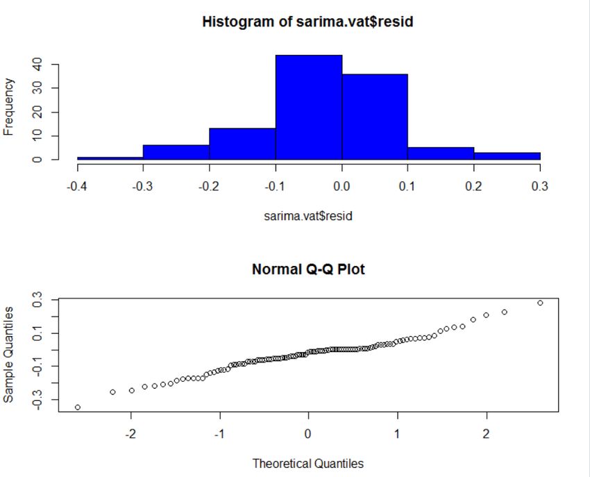
Journal of Economics Library
Table1. Model coefficients and statistics
 1 Θ1
 coef -0.809 -0.582
 s.e. 0.075 0.121
 t ratio -10.749 -4.824
 p-value 6.01E-27 1.41E-06
Source: Author’s computation

 4.3. In-sample measure of accuracy
 Table 2 shows the measure of accuracy on the data for the 14% rate
horizon (the reduced data) to reveal the model performance which can be
referred to as error measurement.

Table 2. SARIMA measure of accuracy
 ME RMSE MAE MPE MAPE MASE
 Error measures -0.03026194 0.1041971 0.07390177 -0.3163756 0.7552092 0.6604111
Source: Author’s computation

 As discussed in section 3.2, the most crucial thing in ARIMA/SARIMA
models is to examine the model residuals in order to identify if they are
distributed normally around zero. This can be achieved through
visualisation of the residuals as shown in figure 2.

 Figure 2. Residuals histogram and Q-Q plot
 Source: Author’s computation

 C.T. Koloane & M.P. Makananisa, 7(3), 2020, p.123-136.
 131

 131

Journal of Economics Library
 The two plots in Figure 2 shows the distribution of the residual
overtime. It can be observed from the plots above that most of the values
are spread around the zero mean. Thus, the residual histogram and the q-q
plot seems to confirm the independence of the residuals.
 The Ljung–Box test with a chi-squared of 21.435 from 20 degrees of
freedom gave a p-value of 0.372 was obtained from the model. This is an
indication of uncorrelated residuals which are assumed to be coming from
a well specified model and for this reason the model will be used to predict
VAT historical payments.
 The model’s good fit on the sample data enables the model to be used
for forecasting purposes with some level of accuracy. Depending on the
tolerance level or error range, the model can be regarded as good. The rule
of thumb error preference is the 5% error rate.
 Table3compares the actual and the model fitted values for the fiscal year
2009/10 to 2017/18. Although the model performance was poor for the years
2010/11 and 2011/12, for the recent years the same model performed much
better at an error rate lower than 5%.

Table 3. Actual and models fitted values in rand million
 FY Actual Fitted % Error
 2009/10 147 943 147 853 0.1%
 2010/11 183 572 202 533 -10.3%
 2011/12 191 021 206 283 -8.0%
 2012/13 215 023 217 136 -1.0%
 2013/14 237 668 240 557 -1.2%
 2014/15 261 295 263 353 -0.8%
 2015/16 281 101 283 135 -0.7%
 2016/17 289 167 297 803 -3.0%
 2017/18 297 992 303 941 -2.0%
Source: South African national treasury and own computation

 4.4. SARIMA model predictions/forecasts
 Table 4 below presents the actual and model prediction for the year
2018/19 and 2019/20 and the difference thereof.

Table 4. Actual and models predicted values in rand million
 FY Actual (at 15%) Prediction (at 14%) Difference(Impact) % Difference
 2018/19 324 765 311 223 13 542 4.2%
 2019/20 346 747 326 703 20 044 5.8%
Source: Author’s computation

 Assuming no change on the 14% VAT rate, the model fitted to the data
predicted the collection of R311.2bn and R326.7bn for 2018/19 and 2019/20
respectively with 5% tolerance (error) level. The difference between
prediction (at 14% rate) and actual realisation of R324.8bn and R346.7bn for
the same period (at 15% rate) was computed to obtain the impact. Based on
the model fitted, a percentage increase in VAT rate increased its payments

 C.T. Koloane & M.P. Makananisa, 7(3), 2020, p.123-136.
 132

 132

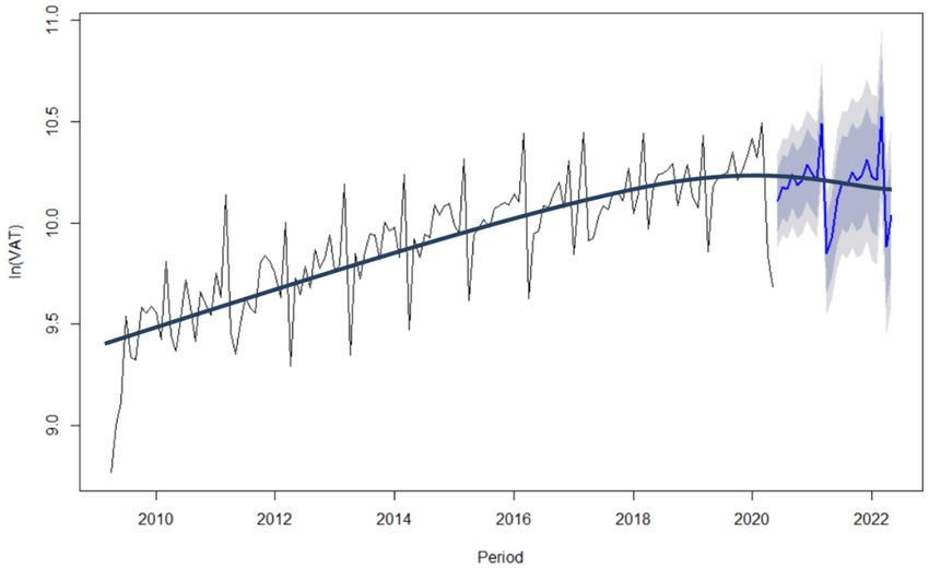
Journal of Economics Library
by 4.2% in 2018/19 and 5.8% in 2019/20. This results in a slight increase in
the total state revenue of 1.1% and 1.5% in 2018/19 and 2019/20
respectively.
 Figure 3 below shows the VAT historical actual and forecast for financial
year 2020/21 at 15% rate. The SARIMA model forecasted R313.9bn to be
collected for the same period. This is lower than the collected net VAT for
the period 2019/20 of R346.7bn by roughly R22bn. The lower collection is
due to the covid-19 impact on revenue collection.

 Figure 3. ln(VAT) and forecast for 2020/21 in rand millions
 Source: Author’s computation

 Table 5 unfold or disaggregate the 2020/21 forecast shown in figure 3 to
monthly and cumulative forecast for the same period the actual for April
and May 2020.Though there was an increase from 14% to 15% in VAT rate,
the pandemic shock overwrites this increase and lowers the VAT collection.

Table 5. Forecast for 2020/21 in rand million
 Point Forecast Cum.
 Month Year
 Forecast Lo 95 Hi 95 Forecast
 Apr 2020 18 777 18 777
 May 2020 16 040 34 817
 Jun 2020 24 503 19 433 30 895 59 320
 Jul 2020 26 314 20 714 33 427 85 634
 Aug 2020 25 970 20 296 33 230 111 604
 Sep 2020 27 967 21 704 36 038 139 571
 Oct 2020 26 514 20 436 34 400 166 085
 Nov 2020 27 228 20 846 35 562 193 313
 Dec 2020 29 318 22 302 38 543 222 631
 Jan 2021 28 106 21 244 37 185 250 737
 Feb 2021 27 200 20 432 36 211 277 938
 Mar 2021 35 964 26 851 48 169 313 902
Source: Author’s computation

 C.T. Koloane & M.P. Makananisa, 7(3), 2020, p.123-136.
 133

 133

Journal of Economics Library
 5. Discussion
 The SARIMA model was used to model the monthly VAT collection
contributing to the total state revenue. It was observed that the models
captured the movement of these taxes with high precision. The monthly
forecast was then aggregated to form SARS fiscal year forecast. These
models are preferred for short term predicting/forecasting hence updating
the model is necessary.
 The measures of accuracy i.e. Mean Error, Root Mean Squared Error,
Mean Absolute Error, Percentage Error, Mean Percentage Error and Mean
Absolute Percentage Error were used to show model strength.
 The SARIMA model was fitted on the 14% rate data. The model
predicted R311.2bn and R326.7bn for 2018/19 and 2019/20, which isa
difference of 4.2% in 2018/19 and 5.8% in 2019/20 compared to the actual
realisation at 15%.
 Generally, the use of the SARIMA model assumes the continuation of
historical patterns but giving more weight to recent occurrences. This
makes the model to be more reliable when short term predictions are made.
However, the SARIMA model performance can be severely affected by
unexpected shocks.
 The Covid-19 pandemic which started to impact the world economy
towards the end of calendar year 2019 impose a challenge on revenue
collection. The unexpected pandemic shock (or outliers) will reduce the
VAT maximum revenue collection for fiscal year 2020/21, resulting in lower
overall collection. Estimates from the IMF, Reserve Bank and Organisation
for Economic Co-operation and Development (OECD) suggest that
economic growth in South Africa will contract by between 6 and 7 percent
in 2020 (National Treasury, 2020). This will negatively affect both VAT on
local consumption of goods and VAT on imports. South Africa has already
seen lower import growth from the last quarter of the 2019/20 fiscal year,
because of restrictions on international trading necessitated by the growth
in COVID-19. This was evident in the top 10 trading countries, particularly
China which makes up 20% of South Africa’s dutiable imports.
 The South African government also imposed a hard lockdown on March
27, which lasted for over 60 days. The lockdown resulted in job losses as
most businesses did not operate and some such as liquor, cigarette,
recreation and restaurants were completely not allowed to operate.
 The SARIMA model forecasted R313.9bn to be collected for 2020/21, a
negative growth in VAT collection of 9.5% for the same period from the
positive growth rate of 6.8% in 2019/20.

 6. Conclusion and recommendations
 A percentage increase in VAT rate increased its payments by 4.2% in
2018/19 and 5.8% in 2019/20. This results in a slight increase in the total
state revenue of 1.1% and 1.5% in 2018/19 and 2019/20 respectively.

 C.T. Koloane & M.P. Makananisa, 7(3), 2020, p.123-136.
 134

 134

Journal of Economics Library
Furthermore, the model forecasts R373.6bn to be collected in 2020/21 at 15%
rate.
 The usage of these type of models will assist the South African
government in their budgetary plans and future decisions by taking into
account more accurate projected VAT collection. However, monitoring of
the model is crucial as the prediction power deteriorates in the long run.
 An increase in the tax rate increases the state tax, as a result government
can fund social programmes and public investments that stimulate
economic growth and development. However, the tax burden can also
initiate or increase tax avoidance resulting in an expansion of the tax gap.
This study recommends the balance between the increase in the tax rates
and social benefits.

 C.T. Koloane & M.P. Makananisa, 7(3), 2020, p.123-136.
 135

 135

Journal of Economics Library
References
Budget Speech, (2018). Accessed 10 April 2020. [Retrieved from].
Edzie-Dadzie, J. (2013). Time series analysis of value added tax revenue collection in Ghana,
 A study conducted in partial fulfilment of the requirements for the degree of Masters of
 Science Industrial Mathematics. Kwame Nkrumah University of Science and Technology.
 Institute of Distance Learning. Accra, Ghana. [Retrieved from].
Erero, J.L. (2015). Effects of increases in value added tax: A dynamic CGE approach,
 Economic Research Southern Africa, Working Papers No.558. [Retrieved from].
Gumbo, V., & Dhliwayo, L. (2018). VAT revenue modelling: The case of Zimbabwe.
 Department of Finance, National University of Science and Technology, Bulawayo,
 Zimbabwe.
Gujarati, D.N. (2003). Basic Econometric. 4thed. New York: McGraw Hill.
Gujarati, D.N., & Porter D.C. (2009). Basic Econometric. 5thed. New York: McGrawHill.
Hyndman, R.J., Makridakis, S., & Wheelwright, S.C. (1998). Forecasting Methods and
 Application. 3rded. USA: John Wiley and Sons.
Legeida, N., & Sologoub, D. (2003). Modeling value added tax (VAT) revenues in a
 transition economy: Case of Ukraine, Institute for Economic Research and Policy Consulting,
 Working Paper No.22. [Retrieved from].
Maindonald, J., & Braun, J. (2003). Data Analysis and Graphics using R: An Example-based
 Approach. Cambridge: Cambridge University Press.
Nandi, B.K., Chaudhury, M., & Hasan, G.Q. (2014). Univariate time series forecasting: A
 study of monthly tax revenue of Bangladesh, Centre for Research and Training, Working
 Paper No.9. [Retrieved from].
National Treasury, (2020). Briefing by national treasury on financial implications of COVID-
 19 on both the economy and budget. Accessed 05 June 2020, [Retrieved from].
Ofori, M.S. (2018). VAT revenue forecasting in Ghana, A study conducted in partial
 fulfilment of the requirements for the degree of MPhil Economics. University of Ghana.
 [Retrieved from].
Okseniuk, O. (2015). Methods of forecasting VAT revenuesfor the state budget of Ukraine,
 Ekonomia Międzynarodowa, 10, 81-94.
Pindyck, R.S., & Rubinfeld, D.L. (1998). Econometric Models and Economic Forecast. 4thed.
 Singapore: McGraw Hill.
Streimikiene, D., Ahmed, R.R., Vveinhardt, J., Ghauri, S.P., & Zahid, S. (2018). Forecasting
 tax revenues using time series techniques – A case of Pakistan, Economic Research, 31(1),
 722-754. doi. 10.1080/1331677X.2018.1442236
Tax Statistics, (2019). Accessed 10 April 2020. [Retrieved from].
Wei, W.S. (2006). Time Series Analysis: Univariate and Multivariate Methods, 2nd ed.Pearson:
 Addison Wesley.
Yurekli, K., Kurunc, A., & Ozturk, F. (2005). Testing the residuals of an ARIMA model on
 the Cekerk stream watershed in Turkey, Turkish Journal of Engineering and Environmental
 Sciences, 29(2), 61-74.

Copyrights
Copyright for this article is retained by the author(s), with first publication rights granted to
the journal. This is an open-access article distributed under the terms and conditions of the
Creative Commons Attribution license (http://creativecommons.org/licenses/by-nc/4.0).

 C.T. Koloane & M.P. Makananisa, 7(3), 2020, p.123-136.
 136

 136