Periodic culling outperforms isolation and vaccination strategies in controlling Influenza A (H5N6) outbreaks in the Philippines
←
→
Page content transcription
If your browser does not render page correctly, please read the page content below
Periodic culling outperforms isolation and vaccination strategies in
                                               controlling Influenza A (H5N6) outbreaks in the Philippines
                                                                      Abel Lucidoa,b , Robert Smith?c , Angelyn Laoa
                                                 a
                                                   Mathematics & Statistics Department, De La Salle University, 2401 Taft Avenue, 0922 Manila,
                                                                                           Philippines
                                                 b
                                                   Department of Science & Technology - Science Education Institute, Bicutan, Taguig, Philippines
                                            c
                                              Department of Mathematics, University of Ottawa, 585 King Edward Ave Ottawa, ON K1S 0S1, Canada
arXiv:2002.10130v1 [q-bio.PE] 24 Feb 2020

                                            Abstract
                                            Highly Pathogenic Avian Influenza A (H5N6) is a mutated virus of Influenza A (H5N1)
                                            and a new emerging infection that recently caused an outbreak in the Philippines. The
                                            2017 H5N6 outbreak resulted in a depopulation of 667,184 domestic birds. In this study,
                                            we incorporate half-saturated incidence in our mathematical models and investigate three
                                            intervention strategies against H5N6: isolation with treatment, vaccination and modified
                                            culling. We determine the direction of the bifurcation when R0 = 1 and show that all the
                                            models exhibit forward bifurcation. We administer optimal control and perform numeri-
                                            cal simulations to compare the consequences and implementation cost of utilizing different
                                            intervention strategies in the poultry population. Despite the challenges of applying each
                                            control strategy, we show that culling both infected and susceptible birds is a better control
                                            strategy in prohibiting an outbreak and avoiding further recurrence of the infection from
                                            the population compared to confinement and vaccination.
                                            Keywords: Influenza A (H5N6), half-saturated incidence, isolation, culling, vaccination,
                                            bifurcation, optimal control

                                            1. Introduction
                                                Avian influenza is a highly contagious disease of birds caused by infection with influenza
                                            A viruses that circulate in domestic and wild birds [1]. Some avian influenza virus subtypes
                                            are H5N1, H7N9 and H5N6, which are classified according to combinations of different virus
                                            surface proteins hemagglutinin (HA) and neuraminidase (NA). This disease is categorized
                                            as either Highly Pathogenic Avian Influenza (HPAI), which causes severe disease in poultry
                                            and results in high death rates, or Low Pathogenic Avian Influenza (LPAI), which causes
                                            mild disease in poultry [1].
                                                As reported by the World Health Organization (WHO) [1], H5N1 has been detected in
                                            poultry, wild birds and other animals in over 30 countries and has caused 860 human cases

                                                Email address: angelyn.lao@dlsu.edu.ph (Angelyn Lao)
                                            Preprint submitted to Elsevier                                                      February 25, 2020
in 16 of these countries and 454 deaths. H5N6 was reported emerging from China in early
May 2014 [2]. H5N6 is a mutated virus of H5N1, which has been spreading in Southeast
Asia since 2003 [3]. Bi et al. reported that H5N6 has replaced H5N1 as one of the dominant
avian influenza virus subtypes in southern China [4]. In August 2017, cases of H5N6 in the
Philippines resulted in the culling of 667,184 chicken, ducks and quails [5, 6].
    Due to possible threat of avian influenza virus to cause a pandemic, several mathematical
models have been developed in order to test control strategies. Several included saturation
incidence, where the rate of infection will eventually saturate, showing that protective mea-
sures have been put into place as the number of infected birds increases [7, 8]. With half-
saturated incidence, it includes the half-saturation constant which pertains to the density of
infected individuals that yields 50% chance of contracting the disease[9]. Some intervention
strategies employed to protect against avian influenza are biosecurity, quarantine, control
in live markets, vaccination and culling. Culling is a widely used control strategy during
an outbreak of avian influenza. Gulbudak et al. utilized a function to represent the culling
rate considering both HPAI and LPAI [10, 11]. The two-host model of Liu and Fang (2015)
showed that screening and culling of infected poultry is a critical measure for preventing
human A(H7N9) infections in the long term [12].
    Emergency vaccination, prophylactic or preventive vaccination, and routine vaccination
are the three vaccination strategies mentioned by the United Nations Food and Agriculture
Organization (UNFAO) [13]. In China, A(H5N1) influenza infection caused severe economic
damage for the poultry industry, and vaccination served a significant role in controlling the
spread of this infection since 2004 [14]. UNFAO and Office International des Epizooties
(OIE) of the World Organization for Animal Health suggested vaccination of flocks should
replace mass culling of poultry as primary control strategy during outbreak [15]. For this
reason, many mathematical models focus on how vaccination could prohibit the spread of
infection.
    The importance of optimal control in modelling infectious diseases has been highlighted
by several recent studies. Agusto used optimal control and cost-effective analysis in a two-
strain avian influenza model [16]. Jung et al. used optimal control in modelling H5N1 in
figuring out the prevention of influenza pandemic [17]. Kim et al. utilized an optimal-control
approach in modelling tuberculosis (TB) in the Philippines [18]. Okosun and Smith? used
optimal control to examine strategies for malaria–schistosomiasis coinfection [19].

2. The models
    We examine three control strategies: isolation, culling and vaccination. Our mathemat-
ical models are in the form of half-saturated incidence (HSI), we take into consideration
the density of infected individuals in the population that yields 50% chance of contracting
avian influenza. We present four mathematical models: a model without control, which
describes the transmission dynamics of avian influenza in bird population (i.e., the avian in-
fluenza virus (AIV) model), and three models obtained from the AIV model by applying the
intervention strategies isolation, vaccination and culling. Mathematical models with half-
saturated incidence are more realistic compared to models with bilinear incidence [8, 20, 21].
                                              2
Description of variables and parameters used in the models are listed in the table in Ap-
pendix A.

2.1. AIV model without intervention strategy

            Figure 1: Schematic diagram of the AIV model with half-saturated incidence.

    In the AIV model without intervention strategy (shown in Fig. 1), the bird population
is divided into sub-populations (represented by compartments): the susceptible birds (S)
and the infected birds (I). The total population of birds are represented by N (t) at time t,
where N (t) = S(t) + I(t). The number of susceptible birds increases through birth rate (Λ)
and reduces through the natural death rate of birds (µ). Infected birds additionally decrease
through the disease-specific death rate caused by the virus (δ).
    The number of susceptible birds who become infected through direct contact is repre-
            βSI
sented by H+I   , which denotes the transfer of the susceptible bird population to the infected
bird population. Note that β is the rate at which birds contract avian influenza and H is
the half-saturation constant, indicating the density of infected individuals in the population
that yields 50% possibility of contracting avian influenza [20]. The saturation effect of the
infected bird population indicates that a very large number of infected may tend to reduce
the number of contacts per unit of time due to awareness of farmers to the disease [7]. In
                                                                                            βSI
Figure 1, the dashed directional arrow from I to the arrow from S to I indicates that H+I
is regulated by I.
    Based on AIV model described above, we have the following system of nonlinear ordinary
differential equations (ODEs):
                                                      βSI
                                    Ṡ = Λ − µS −         ,
                                                     H +I                                  (1)
                                          βSI
                                    I˙ =      − (µ + δ)I.
                                         H +I
2.2. Confinement strategy for infected poultry (isolation model)
    Here, we employ the strategy of confining the infected poultry population (which will
be referred as the isolation strategy) into the AIV model. Several studies concluded that
reducing the contact rate is an effective measure in preventing the spread of infection into
the population [21, 22]. For the isolation model (shown in Fig. 2), we have included the
compartment representing the population of isolated birds that undergoes treatment (T )
and the compartment representing the population of recovered birds (R). We denote the
isolation rate of identified infected birds by ψ and the release of birds from isolation by γ.
                                                3
Figure 2: Schematic diagram of confinement or isolation model with HSI
We apply treatment to birds during isolation so that some birds can be released from
isolation even though they were still infected. The proportion of infected birds that have
been put into isolation and recovered is represented by f ; infected birds that have not
recovered and remained infected are represented by (1 − f ). We did not consider natural
recovery of poultry in our model due to high mortality rate of HPAI virus infection.
The system of ODEs for the isolation model is
βSI
Ṡ = Λ − µS − ,
H +I
βSI
I˙ = + (1 − f )γT − (µ + δ + ψ)I, (2)
H +I
Ṫ = ψI − (µ + δ + γ)T,
Ṙ = f γT − µR.
2.3. Immunization of the poultry population (vaccination model)
Figure 3: Schematic diagram of preventive vaccination model with HSI
Infection-reduction measures can also help in controlling the disease during an out-
break [23]. Aside from isolating infected birds, we also recognize vaccination of suscep-
4tible birds as a control strategy to reduce the number of infected birds. Joob and Viroj [2]
reported the existence and effectiveness of a vaccine for birds with H5N6.
According to UNFAO, prophylactic vaccination (or preventive vaccination) is carried out
if a high risk of virus incursion is identified and early detection or rapid response measures
may not be sufficient [13]. In this view, we modified the vaccination model (presented in [21])
by dividing the birth rate (Λ) depending on the prevalence rate of vaccination (p) as shown
in Fig. 3 [21]. The poultry population prone to H5N6 is divided into two compartments:
the vaccinated birds represented by V and the susceptible or unvaccinated birds denoted
by S. In our vaccination model, we differentiate the immunized group (vaccinated) from
non-immunized group (unvaccinated).
We investigate the effectiveness of the vaccine not only through its reported efficacy
(denoted by φ) but also based on the waning rate of the vaccine (denoted by ω). To
represent the acquired immunity of the vaccinated group, the infectivity of vaccinated birds
is reduced by a factor 1 − φ. The system of ODEs representing the vaccination model is
βSI
Ṡ = (1 − p)Λ + ωV − µS − ,
H +I
βV I
V̇ = pΛ − (µ + ω)V − (1 − φ) , (3)
H +I
βSI βV I
I˙ = + (1 − φ) − (µ + δ)I.
H +I H +I
2.4. Depopulation of susceptible and infected birds (culling model)
Figure 4: Schematic diagram of depopulation or culling model with HSI
During outbreaks of avian influenza, one of the most widely used strategies is depop-
ulation or culling [13]. A total number of 667, 184 chicken, ducks, and quails were culled
in August 2017 to resolve the outbreak of H5N6 in the Philippines [5, 6]. Several studies
employed culling as a control strategy against avian influenza [11, 12, 24, 25] and pointed
out the significance of obtaining an appropriate threshold policy to combat avian influenza
and prevent the overkilling of birds.
The culling models of Gulbudak et al. considered bilinear incidence in transmission of
infection [10, 11]. Gulbudak and Martcheva designated a culling rate for each strategy by
a different function [11]. Gulbudak et al. used half-saturated incidence to represent the
culling rate for the infected population [10]. In our case, we improved their culling model
by incorporating the dynamics of half-saturated incidence on the transmission of infection
5and on the culling rate for infected birds and for susceptible birds that are at high risk of
infection.
Moreover, we define the culling function of the infected and susceptible birds as τi (I) =
ci I cs I
H+I
and τs (I) = H+I , respectively. The culling rate is represented by cs for susceptible birds
and ci for infected birds. The following system of ODEs represents the culling model:
βSI
Ṡ = Λ − µS − τs (I)S − ,
H +I (4)
βSI
I˙ = − (µ + δ)I − τi (I)I.
H +I
3. Stability and bifurcation analysis
We first analyze the AIV model without intervention. The disease-free equilibrium (DFE)
of the AIV model (1) is
0 0 0
Λ
EA = S , I = ,0 .
µ
The basic reproduction number for the AIV model is
βΛ
RA = . (5)
Hµ(µ + δ)
The disease-free equilibrium EA0 of the AIV model is locally asymptotically stable if RA < 1
and unstable if RA > 1.
The endemic equilibrium for the AIV model is represented by
∗ ∗ ∗ Λ + H(µ + δ) βΛ − µH(µ + δ)
EA = (S , I ) = , . (6)
µ+β (µ + δ)(µ + β)
From AIV model, we obtain two possible endemic equilibria, that is EA∗ and
(µ + δ)(H + I1∗ ) Λ − µS1∗
∗ ∗ ∗
EA1 = (S1 , I1 ) = , .
µ+β β − (Λ − µS1∗ )
Simplifying S1∗ and I1∗ will result to EA∗ 1 = EA∗ , and we have an endemic equilibrium. We
can rewrite I ∗ as
µH
I∗ = (RA − 1).
µ+β
Hence when RA ≤ 1 then I ∗ ≤ 0, so there is no biologically feasible endemic equilibrium.
For RA > 1, we have I ∗ > 0, so we have an endemic equilibrium. We conclude that the AIV
model has no endemic equilibrium when RA ≤ 1, and has an endemic equilibrium when
RA > 1. It follows that reducing the basic reproduction number (RA ) below one is sufficient
to eliminate avian influenza from the poultry population.
As exhibited in Fig. 5A, we have a bifurcation plot between the infected population
and the basic reproduction number RA . Clearly, we have a forward bifurcation for the
6Figure 5: Bifurcation diagram for AIV (A), isolation (B), vaccination (C) and culling (D) model with respect
to their basic reproduction number, indicating only forward bifurcations.
AIV model, showing that when the basic reproduction number crosses unity, an endemic
equilibrium appears.
We continue by investigating different strategies that can reduce or stop the spreading
of AIV. From the isolation model (2), the DFE is given by
0 0 0 0 0
Λ
ET = S , I , T , R = , 0, 0, 0 .
µ
The corresponding basic reproduction number (RT ) is represented by
βΛ(µ + δ + γ)
RT = . (7)
Hµ[(µ + δ + ψ)(µ + δ + γ) − (1 − f )γψ]
The disease-free equilibrium (ET0 ) of the isolation model is locally asymptotically stable
if RT < 1 and unstable if RT > 1. Consequently, we can identify some conditions on
how confinement of infected birds affects the stability of ET0 . The DFE (ET0 ) is locally
asymptotically stable whenever
βΛ(µ + δ + γ) − Hµ(µ + δ)(µ + δ + γ)
ψ> .
Hµ(µ + δ + f γ)
For the endemic equilibrium of the isolation model (2), we indicate the presence of
infection in the population by letting I 6= 0 and solve for S, I, T , and R. Thus, we have
ET∗ = (S ∗∗ , I ∗∗ , T ∗∗ , R∗∗ )
Λ(H + I ∗∗ )
[βΛ − µH(µ + δ + ψ)](µ + δ + γ) + (1 − f )γψµH
= ∗∗ ∗∗
, ,
µ(H + I ) + βI (µ + β)[(µ + δ + ψ)(µ + δ + γ) − (1 − f )γψ] (8)
ψI ∗∗ f γψI ∗∗
, .
µ + δ + γ µ(µ + δ + γ)
7Given the basic reproduction number (7), we rewrite the expression I ∗∗ of the isolation
model as
µH(RT − 1)
I ∗∗ = . (9)
µ+β
From (9), it follows that when RT ≤ 1, we have Ib ≤ 0 and there is no endemic equi-
librium; but when RT > 1, we get Ib > 0 and we have an endemic equilibrium. Thus, the
isolation model (2) has no endemic equilibrium when RT ≤ 1 and has an endemic equilib-
rium when RT > 1. Hence there is no backward bifurcation for the isolation model when
RT < 1.
In Fig. 5B, we have a forward bifurcation for the isolation model, which supports our
claim. The bifurcation plot between the infected population I ∗∗ and the basic reproduc-
tion number RT for the isolation model shows that reducing RT below unity is enough to
eliminate avian influenza from the poultry population.
Next we analyze the stability of the associated equilibria of the AIV model with vacci-
nation strategy (3). The DFE and the basic reproduction number are
0 0 0 0 (µ + ω − pµ)Λ pΛ
EV = (S , V , I ) = , ,0
µ(µ + ω) µ+ω
and
Λβ(µ + ω − pµφ)
RV = .
µH(µ + ω)(µ + δ)
The disease-free equilibrium EV0 of vaccination model is locally asymptotically stable if
RV < 1 and unstable if RV > 1. Moreover, we obtain some conditions for the prevalence
rate of vaccination (p) and vaccine efficacy (φ), which both range from 0 to 1. The DFE EV0
of vaccination model is locally asymptotically stable whenever
(µ + ω) µH(µ + δ)
1− ≤ pφ < 1
µ Λβ
For the endemic equilibrium of the vaccination model (3), we obtain the following:
EV∗ = (S ∗∗∗ , V ∗∗∗ , I ∗∗∗ )
(H + I ∗∗∗ )[(1 − p)Λ[(µ + ω)(H + I ∗∗∗ ) + (1 − φ)βI ∗∗∗ ] + ωpΛ(H + I ∗∗∗ )]
= ,
[µ(H + I) + βI][(µ + ω)(H + I ∗∗∗ ) + (1 − φ)βI ∗∗∗ ]
√
pΛ(H + I ∗∗∗ )
−b ± b2 − 4ac
,
(µ + ω)(H + I ∗∗∗ ) + (1 − φ)βI ∗∗∗ 2a
such that
a = −(µ + δ)[µβ(1 − φ) + (µ + ω)(µ + β) + β 2 (1 − φ)],
b = β 2 Λ(1 − φ) + µH(µ + δ)(µ + ω)(RV − 1)
− (µ + δ)H[µβ(1 − φ) + (µ + β)(µ + ω)],
c = µH 2 (µ + δ)(µ + ω)(RV − 1).
8The vaccination model (3) has no endemic equilibrium when RV ≤ 1, and has a unique
endemic equilibrium when RV > 1. Fig. 5C illustrates a bifurcation plot between the
population of infected birds and the basic reproduction number RV , showing a forward
bifurcation. This bifurcation diagram is in line with our result in Theorem Appendix B.1,
so there is no endemic equilibrium when RV < 1, but there is a unique endemic equilibrium
when RV > 1. In this case, reducing RV below one is sufficient to control the disease.
Finally, we analyze the stability of equilibria of the AIV model with culling (4). The
DFE for the culling model is given by
0 0 0
Λ
EC = S , I = ,0 .
µ
and the basic reproduction number is
βΛ
RC = .
Hµ[µ + δ]
The endemic equilibria of the culling model is determined as
√
Λ(H + I ∗∗∗∗ )
−b ± b2 − 4ac
EC∗ = (S ∗∗∗∗
,I ∗∗∗∗
)= , , (10)
µH + (µ + cs + β)I ∗∗∗∗ 2a
such that
a = −(µ + δ + ci )(µ + cs + β),
b = µH(µ + δ)(RC − 1) − ci µH − H(µ + δ)(µ + cs + β),
c = µH 2 (µ + δ)(RC − 1).
For the culling model (4), we have shown that a backward bifurcation does not exist
when RC < 1. The culling model (4) has no endemic equilibrium when RC < 1, and has a
unique endemic equilibrium when RC > 1.
In Fig. 5D, we have a bifurcation diagram showing the infected population and the basic
reproduction number (RC ). We have a forward bifurcation in the plot, which is similar to
the result stated in Theorem Appendix B.2, implying that, when RC < 1, avian influenza
dies out from the poultry population.
4. Optimal control strategies
We now integrate an optimal-control approach in all our models: isolation, vaccination,
and culling.
94.1. Isolation
Our first control involves isolating infected birds with u1 replacing ψ. The second con-
trol indicates the effort of the farmers in choosing a drug that can increase the success of
treatment with u2 replacing f . The isolation model (2) becomes
βSI
Ṡ = Λ − µS − ,
H +I
βSI
I˙ = + (1 − u2 (t)) γT − (µ + δ + u1 (t)) I, (11)
H +I
Ṫ = u1 (t)I − (µ + δ + γ)T,
Ṙ = u2 (t)γT − µR.
We represent the rate of isolation of infected birds by control u1 (t), that is the rate u1 (t)I
transfers from I to T . The proportion of successfully treated birds released from isolation
is denoted by u2 (t).
The problem is to minimize the objective functional defined by
Z tf
B1 2 B2 2
JI (u1 , u2 ) = I(t) + T (t) + u (t) + u (t) dt,
0 2 1 2 2
which is subject to the ordinary differential equations in (11) and where tf is the final time.
The objective functional includes isolation control (u1 (t)) and treatment control (u2 (t)),
while B1 and B2 are weight constants associated to relative costs of applying respective
control strategy. Given that we have two controls u1 (t) and u2 (t), we want to find the
optimal controls u∗1 (t) and u∗2 (t) such that
JI (u∗1 , u∗2 ) = min{JI (u1 , u2 )},
UI
where UI = {(u1 , u2 )| ui : [0, tf ] → [ai , bi ], i = 1, 2, is Lebesgue integrable} is the control set.
We consider the worst and best scenarios of isolating infected birds and giving treatment by
letting the lower bounds ai = 0 and upper bounds bi = 1, for i = 1, 2.
4.1.1. Characterization of optimal control for isolation strategy
We generate the necessary conditions of this optimal control using Pontryagin’s Maxi-
mum Principle [26]. We define the Hamiltonian, denoted by HI , as follows:
B1 2 B2 2 βSI
HI = I(t) + T (t) + u (t) + u (t) + λI1 Λ − µS −
2 1 2 2 H +I
βSI (12)
+ λI2 + [1 − u2 (t)] γT − [µ + δ + u1 (t)] I
H +I
+ λI3 (u1 (t)I − (µ + δ + γ)T ) + λI4 (u2 (t)γT − µR) ,
where λI1 , λI2 , λI3 , λI4 are the associated adjoints for the states S, I, T, R. We obtain the
system of adjoint equations by using the partial derivatives of the Hamiltonian (12) with
respect to each state variable.
10Theorem 4.1. There exists optimal controls u∗1 (t) and u∗2 (t) and solutions S ∗ , I ∗ , T ∗ , R∗ of
the corresponding state system (11) that minimizes the objective functional JI (u1 (t), u2 (t))
over UI . Then there exists adjoint variables λI1 , λI2 , λI3 , and λI4 satisfying
dλI1 βI βI
= λI1 µ + − λI2 ,
dt H +I H +I
dλI2 HβS HβS
= −1 + λI1 − λI2 + λI2 [µ + δ + u1 (t)] − λI3 u1 (t)
dt (H + I)2 (H + I)2
dλI3
= −1 − λI2 [1 − u2 (t)] γ + λI3 (µ + δ + γ) − λI4 u2 (t)γ,
dt
dλI4
= λI4 µ
dt
with transversality conditions λIi (tf ) = 0, for i = 1, 2, 3, 4. Furthermore,
∗ (λI2 − λI3 ) I ∗ (λI2 − λI4 ) γT
u1 = min b1 , max a1 , and u2 = min b2 , max a2 , .
B1 B2
(13)
Proof. The existence of optimal control (u∗1 , u∗2 ) is given by the result of Fleming and Rishel
(1975). Boundedness of the solution of our system (2) shows the existence of a solution for the
system. We have nonnegative values for the controls and state variables. In our minimizing
problem, we have a convex integrand for JI with respect to (u1 , u2 ). By definition, the
control set is closed, convex, and compact which shows the existence of optimality solutions
in our optimal system. By Pontryagin’s Maximum Principle [26], we obtain the adjoint
equations and transversality conditions. We differentiate the Hamiltonian (12) with respect
to the corresponding state variables as follows:
dλI1 ∂HI dλI2 ∂HI dλI3 ∂HI dλI4 ∂HI
=− , =− , =− , =−
dt ∂S dt ∂I dt ∂T dt ∂R
with λIi (tf ) = 0 where i = 1, 2, 3, 4. We consider the optimality condition
∂HI ∂HI
= B1 u1 (t) − λI2 I + λI3 I = 0 and = B2 u2 (t) − λI2 γT + λI4 γT = 0
∂u1 ∂u2
to derive the optimal controls in (13). We consider the bounds of the controls and obtain
the characterization for optimal controls u∗1 and u∗2 as follows:
(λI2 − λI3 ) I (λI2 − λI4 ) γT
u∗1 = min 1, max 0, and u∗2 = min 1, max 0, .
B1 B2
114.2. Vaccination
For vaccination, the first control represents the effort of the farmers to increase vaccinated
birds, while the other control describes the efficacy of the vaccine in providing immunity
against H5N6. Where u3 (t) and u4 (t) replace p and φ, respectively, into the vaccination
model (3) to obtain
βSI
Ṡ = (1 − u3 (t)) Λ + ωV − µS − ,
H +I
βV I
V̇ = u3 (t)Λ − (µ + ω)V − [1 − u4 (t)] , (14)
H +I
βSI βV I
I˙ = + [1 − u4 (t)] − (µ + δ)I.
H +I H +I
We describe the proportion of birds that are vaccinated by the control u3 (t) and the
immunity of the vaccinated population against acquiring the disease by u4 (t).
We have the objective functional
Z tf
B3 2 B4 2
JV (u3 , u4 ) = I(t) + u (t) + u (t) dt,
0 2 3 2 4
which is subject to (3). This objective functional involves increased vaccination u3 (t) and
the vaccine-efficacy control u4 (t), where B3 and B4 are the weight constants representing the
relative cost of implementing each respective controls. We need to find the optimal controls
u∗3 (t) and u∗4 (t) such that
JV (u∗3 , u∗4 ) = min{JV (u3 , u4 )},
UV
where UV = {(u3 , u4 )|ui : [0, tf ] → [ai , bi ], i = 3, 4, is Lebesgue integrable} is the control
set. We consider the lower bound ai = 0 and upper bounds bi = 1, for i = 3, 4.
4.2.1. Characterization of optimal control for vaccination strategy
Similarly, we use Pontryagin’s Maximum Principle [26] to show necessary conditions of
optimal control. We define the Hamiltonian denoted by HV as follows:
B3 2 B4 2 βSI
HV = I(t) + u (t) + u (t) + λV1 (1 − u3 (t))Λ + ωV − µS −
2 3 2 4 H +I
βV I
+ λV2 u3 (t)Λ − (µ + ω)V − (1 − u4 (t)) (15)
H +I
βSI βV I
+ λV3 + [1 − u4 (t)] − (µ + δ)I .
H +I H +I
Theorem 4.2. There exists optimal controls u∗3 (t) and u∗4 (t) and solutions S ∗ , V ∗ , I ∗ of the
corresponding state system (14) that minimize the objective functional JV (u3 (t), u4 (t)) over
12UV . Then there exists adjoint variables λV1 , λV2 and λV3 satisfying
dλV1 βI βI
= λV1 µ + − λV3 ,
dt H +I H +I
dλV2 βI βI
= − λV1 ω + λV2 µ + ω + [1 − u4 (t)] − λV3 [1 − u4 (t)] ,
dt H +I H +I
dλV3 HβS HβV
= − 1 + λV1 + λV2 [1 − u4 (t)]
dt (H + I)2 (H + I)2
HβS HβV
− λV3 + [1 − u4 (t)] − (µ + δ) ,
(H + I)2 (H + I)2
with transversality conditions λVi (tf ) = 0, for i = 1, 2, 3. Furthermore,
∗ (λV1 − λV2 ) Λ ∗ (λV3 − λV2 ) βV I
u3 = min b3 , max a3 , and u4 = min b4 , max a4 , .
B3 B4 (H + I)
(16)
Proof. Similarly, the existence of optimal control (u∗3 , u∗4 ) is given by the result of Fleming
and Rishel (1975). Boundedness of the solution of our system (3) shows the existence of a
solution for the system. We have nonnegative values for the controls and state variables.
In our minimizing problem, we have a convex integrand for JV with respect to (u3 , u4 ).
By definition, the control set is closed, convex, and compact which shows the existence of
optimality solutions in our optimal system. We use Pontryagin’s Maximum Principle [26] to
obtain the adjoint equations and transversality conditions. We differentiate the Hamiltonian
(15) with respect to the corresponding state variables as follows:
dλV1 ∂HV dλV2 ∂HV dλV3 ∂HV
=− , =− , =−
dt ∂S dt ∂V dt ∂I
with λVi (tf ) = 0 where i = 1, 2, 3. Using the optimality condition
∂HV ∂HV βV I βV I
= B3 u3 (t) − λV1 Λ + λV2 Λ = 0 and = B4 u4 (t) + λV2 − λV3 = 0.
∂u3 ∂u4 H +I H +I
we derive the optimal controls (16). We consider the bounds for the control and conclude
the characterization for u∗3 and u∗4
(λV1 − λV2 ) Λ (λV3 − λV2 ) βV I
u∗3 = min 1, max 0, and u∗4 = min 1, max 0, .
B3 B4 (H + I)
134.3. Culling
Finally, we administer optimal control to the culling model (4). Thus we have
u5 (t)SI βSI
Ṡ = Λ − µS − − ,
H +I H +I
(17)
βSI u6 (t)I 2
I˙ = − (µ + δ)I − .
H +I H +I
We represent the frequency of culling the susceptible population by u5 (t) and frequency
of culling the infected population by u6 (t). We have the objective functional
Z tf
B5 2 B6 2
JC (u5 , u6 ) = I(t) + u (t) + u (t) dt,
0 2 5 2 6
which is subject to (4). The objective functional includes the susceptible and infected culling
control denoted by u5 (t) and u6 (t), respectively, with B5 and B6 as the weight constants
representing the relative cost of implementing each respective controls. Hence we have to
find the optimal controls u∗5 and u∗6 such that
JC (u∗5 , u∗6 ) = min{JC (u5 , u6 )},
UV
where UC = {(u5 , u6 )|[0, tf ] → [ai , bi ], i = 5, 6, is Lebesgue integrable} is the control set.
We consider the lower bound ai = 0 and upper bounds bi = 1, for i = 5, 6.
4.3.1. Characterization of optimal control for culling strategy
We utilize the Pontryagin’s Maximum Principle [26] to show the necessary conditions of
optimal control. We define the Hamiltonian denoted by HC as follows:
B5 2 B6 2 u5 (t)SI βSI
HC = I(t) + u (t) + u (t) + λC1 Λ − µS − −
2 5 2 6 H +I H +I
2
(18)
βSI u6 (t)I
+ λC2 − (µ + δ)I − .
H +I H +I
Theorem 4.3. There exists optimal controls u∗5 (t) and u∗6 (t) and solutions S ∗ , I ∗ of the
corresponding state system (17) that minimize the objective functional JC (u5 (t), u6 (t)) over
UC . Then there exists adjoint variables λC1 and λC2 satisfying
dλC1 u5 (t)I βI βI
= λC1 µ + + − λC2 ,
dt H +I H +I H +I
dλC2 u5 (t)HS HβS HβS (2H + I)u6 (t)I
= −1 + λC1 + − λC2 − (µ + δ) −
dt (H + I)2 (H + I)2 (H + I)2 (H + I)2
with transversality conditions λCi (tf ) = 0 for i = 1, 2. Furthermore,
λC2 I 2
∗ λC1 SI ∗
u5 = min b5 , max a5 , and u6 = min b6 , max a6 , .
B5 (H + I) B6 (H + I)
(19)
14Proof. The existence of optimal control (u∗5 , u∗6 ) is given by the result of Fleming and Rishel
(1975). Boundedness of the solution of our system (4) shows the existence of a solution for the
system. We have nonnegative values for the controls and state variables. In our minimizing
problem, we have a convex integrand for JC with respect to (u5 , u6 ). By definition, the
control set is closed, convex, and compact which shows the existence of optimality solutions
in our optimal system. By Pontryagin’s Maximum Principle [26], we obtain the adjoint
equations and transversality conditions. We differentiate the Hamiltonian (18) with respect
to the corresponding state variables as follows:
dλC1 ∂HC dλC2 ∂HC
=− and =−
dt ∂S dt ∂I
with λCi (tf ) = 0 where i = 1, 2. We consider the optimality condition
∂HC λC SI ∂HC λC2 I 2
= B5 u5 (t) − 1 = 0 and = B6 u6 (t) − = 0,
∂u5 H +I ∂u6 H +I
to derive the optimal controls (19). We consider the bounds of the controls and get the
characterization for u∗5 and u∗6
λC2 I 2
∗ λC1 SI ∗
u5 = min 1, max 0, and u6 = min 1, max 0, .
B5 (H + I) B6 (H + I)
5. Numerical simulations
The parameter values applied to generate our simulations are listed in the table in the
appendix. The initial conditions of the simulations are based on the Philippines’ H5N6
outbreak report given by the OIE [27]. We set S(0) = 407 837, I(0) = 73 360, T (0) = 0,
R(0) = 0, and the total population of birds N (0) = 481 197.
Previous studies suggested that the basic reproduction number for the presence of avian
influenza without applying any intervention strategy is RA = 3 [28, 29]. Given this as-
sumption, we have calculated the transmissibility of the disease (β = 0.025) based on (5).
Without any control strategy, avian influenza will become endemic in the poultry population
as shown in Fig. 6. After 50 days, the population of the infected poultry exceeds that of
susceptible poultry, with all birds eventually infected or dead.
Figs. 7–9 illustrate the effects of applying optimal control to isolation strategy under
different approaches. These simulations suggest that isolation must be complemented by
treatment, where the cheaper cost of implementation works best since it will enable us to
apply the strategy in to a larger population of poultry. Application of optimal controls u∗1 (t)
and u∗2 (t) in the susceptible, infected, isolated and recovered population is clearly better
than the absence of optimal control (Fig. 7). We can observe a slower decline of susceptible
birds, an initial reduction in infected birds and a delayed increase in infection. More infected
birds are isolated (Fig. 7C), and we have a higher number of birds that will recover after
going through isolation (Fig. 7D).
15Figure 6: Simulation results showing the transmission dynamics of H5N6 in the Philippines with no inter-
vention strategy. We use initial conditions and parameter values as follows: S(0) = 407 837, I = 73 360,
Λ = 2365
060
, µ = 3.4246 × 10⁻⁴ , β = 0.025, H = 180 000, δ = 4 × 10⁻⁴
A cheaper relative cost of implementing both controls u1 (t) and u2 (t) leads to lower
infected populations, as illustrated in Fig. 8. We can observe that when we have lower values
for B1 and B2 , the susceptible population has a slower decline, there are fewer infected and
isolated birds, and there are more recovered birds. Thus, the cheaper controls are more
effective in implementing both isolation and treatment controls.
It is evident that using isolation together with treatment showed better results in all
populations compared to implementing isolation alone, as depicted in Fig. 9. In applying
both controls, the susceptible populations decrease slowly; infected birds are eliminated from
the poultry population; and isolated birds increase within 5 days, then decrease afterward.
This is due to the release of the birds and the effect of treatment where most of the isolated
birds are transferred to the recovered population. Without treatment isolated birds increase
continuously then decrease after 85 days, as illustrated in Fig. 9C. The birds were released
from isolation zone even though they are still infectious. Our results suggest that the
isolation strategy can be maximized by administering isolation together with treatment.
Empirically, we have found that, through the application of optimal control to isolation
with treatment strategy, it is possible to control an outbreak, as shown in the numerical
simulation from Figs. 7–9. This also suggests that isolation is more effective if utilized
together with treatment. In addition, a cheaper cost of applying both isolation control and
treatment control will result in a lower infected population and more recovered birds.
Through the application of optimal-control approach in vaccination, we can observe that
the diminishing effectiveness of the vaccine results to spread of infection in the vaccinated
population, as depicted in Fig. 10. After 150 days, the vaccine efficacy started to decline
causing vaccinated birds to acquire the disease. While in Fig. 11, taking a lower value for
both B3 and B4 provides a higher vaccine efficacy resulting to a higher susceptible and
vaccinated population. Hence, for using vaccination strategy, we need to consider cheap
vaccine that sustains its effectiveness in a longer period.
Simulations shown in Figs. 10–11 contribute to our understanding that providing immu-
16Figure 7: Applying the isolation strategy with (blue solid line) and without (red dashed line) optimal control
in the population of susceptible (A), infected (B), isolated (C) and recovered (D) birds.
nity to the poultry population is not sufficient to prevent an outbreak due to the possibility
of the vaccine to lose its effectiveness. In using an optimal-control approach, we see that a
successful immunization strategy highly depends on choosing a long-lasting and an effective
vaccine.
Integrating optimal control into a culling strategy results in a lower population for both
susceptible and infected birds as compared to using fixed control, as portrayed in Fig. 12.
We notice that the decline in the numbers of both susceptible and infected birds occurs
faster when optimal control is applied. Culling strategy with cheaper implementation cost
results to a lesser infected population while susceptible population will be in the same level
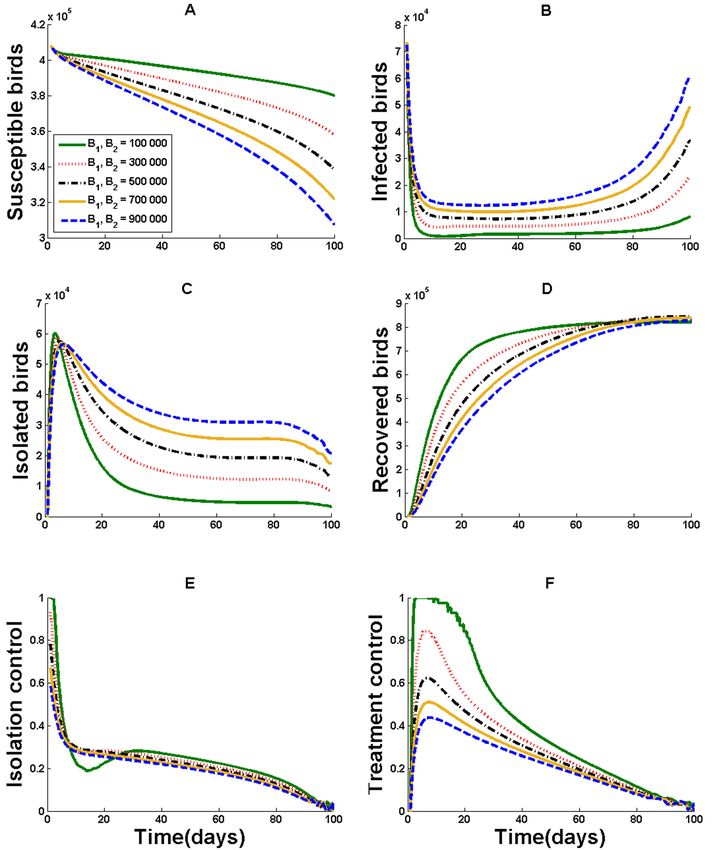
regardless of the implementation cost, as illustrated in Fig. 13.
Fig. 13C–D suggests that high culling frequency for both susceptible and infected popu-
lations are needed in order to prevent an outbreak. Culling frequency for susceptible birds
must be at least 0.30 per day or three times for the first 10 days of the outbreak. The culling
frequency for infected birds must be around 0.15–0.6 per day or 2–6 times for the first 10
days and must stay at 0.1–0.3 per day to keep the number of infected birds low.
Administering a culling strategy for both susceptible and infected birds is more effective
than culling only the infected birds, as indicated in Fig. 14. Looking at the blue dashed
line of Fig. 14A, we have more susceptible birds if we cull only the infected population, but,
as shown in Fig. 14B, the number of infected birds increases afterward. This implies that
culling only the infected population is not enough to stop the spread of infection. We can
infer that culling only the infected population can only be successful if we can eradicate
the infected population. Currently, we cannot easily identify infected birds from the poultry
17Figure 8: Application of isolation with optimal control to the population of susceptible (A), infected (B),
isolated (C) and recovered (D) birds along with isolation control (E) and treatment control (F) for varying
values of Bi , for i= 1,2, from 100, 000 to 900, 000
population. Culling both susceptible and infected birds led to near eradication of the infected
population, and, due to the low number of susceptible birds, further spread of H5N6 would
not be possible. Thus, culling both susceptible and infected birds is necessary to eliminate
the spread of infection in the poultry population.
6. Conclusion
The control strategies we considered include isolation and treatment of infected birds (iso-
lation model), preventive vaccination of poultry (vaccination model), and modified culling
of infected and susceptible birds that are at high risk of infection (culling model). In the
model where isolation and treatment of infected birds is used as strategy, we extended pre-
vious models by considering that some birds that were released from confinement did not
recover successfully. In using preventive vaccination, we also included the waning effect of
the vaccine (in the model). For the model that depopulates the infected and susceptible
18Figure 9: Isolation strategy with the optimal approach and with consideration of using both isolation and
treatment control (blue solid line) and using isolation control (red dashed line) only to the population of
susceptible (A), infected (B), isolated (C) and recovered (D) birds.
birds that are high-risk to infection, we represented culling rate function with respect to
half-saturated incidence.
Our results suggest that, when the basic reproduction number (RA , RT , RV , and RC ) for
each model is below unity, then the disease-free equilibrium is locally asymptotically stable.
All four mathematical models presented here exhibited a forward bifurcation (Fig. 5), so
lowering the basic reproduction number below 1 is sufficient to eliminate H5N6 from the
poultry population.
In applying the optimal-control approach in the isolation strategy, we showed that iso-
lation alone cannot prevent the spread of infection. Instead, it needs to be coupled with
treatment so that the isolated birds can recover and heal from the infection. Figs. 10–11
depict the importance of vaccine efficacy for a vaccination strategy to succeed in hindering
the spread of H5N6.
Depopulating the whole poultry population or mass culling during an outbreak is unac-
ceptable for ethical, ecological and economic reasons [15]. However, various culling strategies
have been considered by several studies, where they obtained that a threshold policy for
culling can prevent overkilling of birds [10, 11, 24]. In this work, we examine the modified
culling strategy, which includes depopulation of not only infected birds but also susceptible
birds that are at high risk of infection. The depopulation of both susceptible and infected
birds is an effective strategy to put an end to the spreading of avian influenza (as shown
in Figs. 12-14). Through application of optimal control to the culling strategy, we suggest
culling at least three times during the first 10 days of the outbreak.
Computing the basic reproduction number can contribute to decision-making in order to
19Figure 10: Applying the vaccination strategy with (blue solid line) and without (red dashed line) optimal
control in the population of susceptible (A), vaccinated (B) and infected (C) birds, together with the
respective values of the increased vaccination (D) and vaccine-efficacy control (E) over time.
identify which parameters will help in inhibiting the transmission of H5N6. By applying the
optimal-control approach to different intervention strategies against H5N6, we have shown
that culling of both infected and susceptible birds that are at high risk of infection is a better
control strategy in prohibiting an outbreak and avoiding further recurrence of the infection
from the population than confinement and vaccination. Every intervention strategy against
H5N6 has advantages and disadvantages, but proper execution and appropriate application
is a significant factor in achieving a desirable outcome.
Acknowledgment
Lucido acknowledges the support of the Department of Science and Technology-Science
Education Institute (DOST-SEI), Philippines for the ASTHRDP Scholarship grant. Lao
holds research fellowship from De La Salle University. RS? is supported by an NSRC Dis-
covery Grant. For citation purposes, please note that the question mark in “Smith?” is part
of his name.
References
[1] WHO, Influenza (Avian and other zoonotic) (2018).
[2] B. Joob, W. Viroj, H5n6 influenza virus infection, the newest influenza, Asian Pacific Journal of Tropical
Biomedicine 5 (6) (2015) 434–437. doi:10.1016/j.apjtb.2015.03.001.
[3] Analysis: H5n6 avian influenza strain can easily spread from bird to bird, Mainichi Daily News (Nov.
2016).
[4] Y. Bi, Q. Chen, Q. Wang, et al., Genesis, Evolution and Prevalence of H5n6 Avian Influenza Viruses
in China, Cell Host Microbe 20 (6) (2016) 810–821. doi:10.1016/j.chom.2016.10.022.
20Figure 11: Application of vaccination strategy with optimal control to the population of susceptible (A),
vaccinated (B) and infected (C) birds and the increased vaccination (D) and the vaccine-efficacy control (E)
with varying values of Bi , for i= 3,4, from 100, 000 to 900, 000.
Figure 12: Implementing the culling strategy with optimal control (blue solid line) and without optimal
control (red dashed line) in the population of susceptible (A) and infected (B) birds.
[5] Culling of poultry animals in 3 quarantine zones completed; Australia identifies avian flu strain as
H5N6 (2017).
[6] President assures Pinoys it’s safe to eat poultry; releases funds for affected poultry farmers (2017).
[7] V. Capasso, G. Serio, A generalization of the Kermack-McKendrick deterministic epidemic model,
Mathematical Biosciences 42 (1) (1978) 43–61. doi:10.1016/0025-5564(78)90006-8.
[8] S. Liu, L. Pang, S. Ruan, X. Zhang, Global Dynamics of Avian Influenza Epidemic Models with
Psychological Effect (2015). doi:10.1155/2015/913726.
[9] Z. Shi, X. Zhang, D. Jiang, Dynamics of an avian influenza model with half-saturated incidence -
ScienceDirect, Applied Mathematics and Computation 355 (2019) 399–416.
[10] H. Gulbudak, J. Ponce, M. Martcheva, Coexistence caused by culling in a two-strain avian influenza
model, Preprint, J. Biol Dynamics 367 (1) (2014) 1–22.
[11] H. Gulbudak, M. Martcheva, Forward hysteresis and backward bifurcation caused by culling in an avian
influenza model, Mathematical Biosciences 246 (1) (2013) 202–212. doi:10.1016/j.mbs.2013.09.001.
[12] Z. Liu, C.-T. Fang, A modeling study of human infections with avian influenza A H7n9 virus in mainland
China, International Journal of Infectious Diseases 41 (2015) 73–78. doi:10.1016/j.ijid.2015.11.
21Figure 13: Application of culling strategy with optimal control to the population of susceptible (A) and
infected (B) birds and susceptible culling control (C) and infected culling control (D) with varying values of
Bi , for i= 5,6, from 100, 000 to 900, 000.
003.
[13] FAO, The Global Strategy for Prevention and Control of H5n1 Highly Pathogenic Avian Influenza
(2007).
[14] H. Chen, Avian influenza vaccination: the experience in China, Revue Scientifique et Technique de
l’OIE 28 (1) (2009) 267–274. doi:10.20506/rst.28.1.1860.
[15] D. Butler, Vaccination will work better than culling, say bird flu experts, Nature 434 (2005) 810.
[16] F. B. Agusto, Optimal isolation control strategies and cost-effectiveness analysis of a two-strain avian
influenza model, Biosystems 113 (3) (2013) 155–164. doi:10.1016/j.biosystems.2013.06.004.
[17] E. Jung, S. Iwami, Y. Takeuchi, T.-C. Jo, Optimal control strategy for prevention of avian influenza
pandemic, Journal of Theoretical Biology 260 (2) (2009) 220–229. doi:10.1016/j.jtbi.2009.05.031.
[18] S. Kim, A. A. de los Reyes, E. Jung, Mathematical model and intervention strategies for mitigating
tuberculosis in the Philippines, Journal of Theoretical Biology 443 (2018) 100–112. doi:10.1016/j.
jtbi.2018.01.026.
[19] K. O. Okosun, R. Smith?, Optimal control analysis of malaria–schistosomiasis co-infection dynamics,
Mathematical Biosciences and Engineering 14 (2017) 377–405.
[20] N. S. Chong, J. M. Tchuenche, R. J. Smith?, A mathematical model of avian influenza with half-
saturated incidence, Theory Biosci. 133 (1) (2014) 23–38. doi:10.1007/s12064-013-0183-6.
[21] H. Lee, A. Lao, Transmission dynamics and control strategies assessment of avian influenza A (H5n6)
in the Philippines, Infectious Disease Modelling 3 (2018) 35–59. doi:10.1016/j.idm.2018.03.004.
[22] Y. Teng, D. Bi, X. Guo, D. Hu, D. Feng, Y. Tong, Contact reductions from live poultry market closures
limit the epidemic of human infections with H7n9 influenza, Journal of Infection 76 (3) (2018) 295–304.
doi:10.1016/j.jinf.2017.12.015.
[23] A. B. Gumel, Global dynamics of a two-strain avian influenza model, International Journal of Computer
Mathematics 86 (1) (2009) 85–108. doi:10.1080/00207160701769625.
[24] N. S. Chong, B. Dionne, R. Smith?, An avian-only Filippov model incorporating culling of both
susceptible and infected birds in combating avian influenza, J. Math. Biol. 73 (3) (2016) 751–784.
doi:10.1007/s00285-016-0971-y.
[25] N. S. Chong, R. J. Smith?, Modeling avian influenza using Filippov systems to determine culling
22Figure 14: Simulation of culling strategy with the optimal approach and with consideration of using both
susceptible culling control u5 (t) and infected culling control u6 (t) (black solid line), using susceptible culling
control u5 (t) only (red dotted-dashed line), and using infected culling control u6 (t) to the population of
susceptible (A) and infected (B) birds.
of infected birds and quarantine, Nonlinear Analysis: Real World Applications 24 (2015) 196–218.
doi:10.1016/j.nonrwa.2015.02.007.
[26] L. S. Pontryagin, V. Boltyanskii, R. Gamkrelidze, E. Mishchenko, Mathematical Theory of Optimal
Processes - CRC Press Book (1986).
[27] OIE World Animal Health Information System (2018).
[28] C. E. Mills, J. M. Robins, M. Lipsitch, Transmissibility of 1918 pandemic influenza, Nature 432 (7019)
(2004) 904–906. doi:10.1038/nature03063.
[29] M. P. Ward, D. Maftei, C. Apostu, A. Suru, Estimation of the basic reproductive number (R0) for
epidemic, highly pathogenic avian influenza subtype H5n1 spread, Epidemiology & Infection 137 (2)
(2009) 219–226. doi:10.1017/S0950268808000885.
[30] S. Liu, S. Ruan, X. Zhang, Nonlinear dynamics of avian influenza epidemic models, Mathematical
Biosciences 283 (2017) 118–135.
23Appendix A. Variables and parameters
Here, we describe each variable and parameter that we used in the AIV model, isolation
model, vaccination model, and culling model.
Notation Description or Label
S(t) Susceptible birds
I(t) Infected birds
T (t) Isolated birds
R(t) Recovered birds
V (t) Vaccinated birds
N (t) Total bird population
Λ Constant birth rate of birds
µ Natural death rate of birds
β Rate at which birds contract avian influenza
H Half-saturation constant for birds
δ Additional disease death rate due to avian influenza
p Prevalence rate of the vaccination program
φ Efficacy of the vaccine
ω Waning rate of the vaccine
ψ Isolation rate of identified infected birds
γ Releasing rate of birds from isolation
f Proportion of recovered birds from isolation
cs Culling frequency for susceptible birds
ci Culling frequency for infected birds
τs (I) Culling rate of susceptible birds
τi (I) Culling rate of infected birds
The initial conditions are based on Philippine Influenza A (H5N6) outbreak report given
by the OIE [27] together with the assumed parameter values.
Appendix B. Non-existence of backward bifurcation
Appendix B.1. Vaccination
In showing
√ that backward bifurcation does not exist for the vaccination model, we have
−b ± b2 − 4ac
I ∗∗∗ =
2a
where
a = −(µ + δ)[µβ(1 − φ) + (µ + ω)(µ + β) + β 2 (1 − φ)],
b = β 2 Λ(1 − φ) + µH(µ + δ)(µ + ω)(RV − 1)
(B.1)
− (µ + δ)H[µβ(1 − φ) + (µ + β)(µ + ω)],
c = µH 2 (µ + δ)(µ + ω)(RV − 1).
24Definition Symbol Value Source
2 060
Constant birth rate of birds Λ per day
365
[24]
Natural mortality rate µ 3.4246 × 10⁻⁴ per day [30]
Transmissibility of the disease β 0.025 per day Assumed
Half-saturation constant for birds H 180 000 birds [21]
Disease induced death rate of poultry δ 4 × 10⁻⁴ per day [30]
Prevalence rate of vaccination program p 0.50 Assumed
Vaccine efficacy φ 0.90 Assumed
Waning rate of the vaccine ω 0.00001 per day Assumed
Isolation rate of identified infected birds ψ 0.01 per day Assumed
Releasing rate of birds from isolation γ 0.09 per day Assumed
Proportion of fully-recovered birds from isolation f 0.50 Assumed
1
Culling frequency for susceptible birds cs 60
per day Assumed
1
Culling frequency for infected birds ci 7
per day Assumed
Theorem Appendix B.1. The vaccination model (3) has no endemic equilibrium when
RV ≤ 1, and has a unique endemic equilibrium when RV > 1.
Proof. We obtain two possible endemic equilibria EV∗1 and EV∗2 for the vaccination model.
From (B.1), we establish the relationship between RV and c such that
RV > 1 ⇔ c > 0, RV = 1 ⇔ c = 0, RV < 1 ⇔ c < 0
From (B.1), it is clear that a < 0. Now, we consider the following case when c > 0, when
b > 0 and c = 0 or (b2 − 4ac) = 0, and when c < 0, b > 0, and (b2 − 4ac) > 0.
Case 1: c > 0
When c > 0, we have RV > 1. Since a < 0, it follows that
√ √
−b + b2 − 4ac −b − b2 − 4ac
I1∗∗∗ = 0
2a 2a
and when RV > 1 the infected population (I1∗∗∗ ) of the endemic equilibrium (EV∗1 ) does
not exist and we have a unique endemic equilibrium EV∗2 .
Case 2: b > 0 and either c = 0 or b2 − 4ac = 0
Given that b > 0, we consider the case when c = 0 and when b2 − 4ac = 0.
Case 2A: c = 0
Since c = 0 then I1∗∗∗ = 0 and I2∗∗∗ > 0. Note that I1 = 0 leads to the disease-free equilib-
rium. Hence, if b > 0 and c = 0 then I2∗∗∗ > 0 and we have a unique endemic equilibrium EV∗2 .
25Case 2B: b2 − 4ac = 0
Considering that b2 − 4ac = 0, it follows that I1∗∗∗ = I2∗∗∗ and I1∗∗∗ , I2∗∗∗ > 0. Thus, if b > 0
and b2 − 4ac = 0, then we have a unique endemic equilibrium EV∗∗∗ 1
= EV∗∗∗
2
.
Case 3: c < 0, b > 0, and b2 − 4ac > 0
From the assumption that a < 0 and c < 0, it follows that
√ √
∗∗∗ −b + b2 − 4ac ∗∗∗ −b − b2 − 4ac
I1 = >0 I2 = > 0.
2a 2a
Thus, we have two endemic equilibria I1∗∗∗ and I2∗∗∗ which implies that backward bifurcation
may possibly occur whenever c < 0, b > 0, and b2 − 4ac > 0.
However, given the values of b and c, we can show that when c < 0 we cannot obtain
b > 0 which we prove by contradiction. Suppose that c < 0 and by definition of p and φ,
the value of both parameters ranges from 0 to 1, that is 0 ≤ p ≤ 1 and 0 ≤ φ ≤ 1. So, from
µH∆
(B.1) it follows that Λβ < where we define Θ = (µ + ω − pµφ) and ∆ = (µ + δ)(µ + ω).
Θ
Using (B.1) with b > 0 we get Λβ 2 (1 − φ) + ΛβΘ > 2µH∆ + βH∆ + µHβ(µ + δ)(1 − φ).
By simplifying, we obtain
µβ(µ + ω)(1 − φ)
> µ(µ + ω) + β(µ + ω) + µβ(1 − φ). (B.2)
Θ
As mentioned above 0 ≤ φ ≤ 1, so we consider the minimum and maximum value of φ
into the inequality in (B.2).
Case 3A: Let φ = 0.
Assuming that φ = 0 so that Θ = (µ + ωb ) and we simplify (B.2) as follows:
0 > µ(µ + ω) + β(µ + ω).
Since all the parameter µ, ω, β ≥ 0, it implies that 0 ≤ µ(µ + ω) + β(µ + ω). Thus, we
have a contradiction. Hence, for φ = 0 and when c < 0 it follows that b ≯ 0.
Case 3B: Let φ = 1.
When φ = 1, we can simplify (B.2) into
0 > µH∆ + βH∆.
Similarly, given that the parameter µ, H, ω, δ, and β ≥ 0, it signifies that we have a
contradiction. Thus, when φ = 1 and c < 0 then b ≯ 0.
From Case 3A and Case 3B, we have shown that for all values of φ as it ranges from 0
to 1, b ≯ 0 whenever c < 0. Results above suggest that two endemic equilibria does not
exist when RV < 1, since the condition c < 0, b > 0, and b2 − 4ac > 0, cannot be satisfied.
From Cases 1 to 3, it is evident that the vaccination model has no endemic equilibrium when
RV < 1 and a unique endemic equilibrium when RV ≥ 1.
26You can also read