An Alternative Lifetime Model for White Light Emitting Diodes under Thermal-Electrical Stresses - MDPI
←
→
Page content transcription
If your browser does not render page correctly, please read the page content below
materials
Article
An Alternative Lifetime Model for White Light
Emitting Diodes under Thermal–Electrical Stresses
Xi Yang, Bo Sun      ID
                          , Zili Wang, Cheng Qian   ID
                                                         , Yi Ren   ID
                                                                         , Dezhen Yang and Qiang Feng *   ID

 School of Reliability and Systems Engineering, Beihang University, Beijing 100191, China;
 bryantyx@buaa.edu.cn (X.Y.); sunbo@buaa.edu.cn (B.S.); wzl@buaa.edu.cn (Z.W.); cqian@sklssl.org (C.Q.);
 renyi@buaa.edu.cn (Y.R.); dezhenyang@buaa.edu.cn (D.Y.)
 * Correspondence: fengqiang@buaa.edu.cn; Tel.: +86-10-82313214

 Received: 12 April 2018; Accepted: 14 May 2018; Published: 16 May 2018

 Abstract: The lifetime prediction using accelerated degradation test (ADT) method has become a
 main issue for white light emitting diodes applications. This paper proposes a novel lifetime model
 for light emitting diodes (LEDs) under thermal and electrical stresses, where the junction temperature
 and driving current are deemed the input parameters for lifetime prediction. The features of LEDs’
 lifetime and the law of lumen depreciation under dual stresses are combined to build the lifetime
 model. The adoption of thermal and electrical stresses overcomes the limitation of single stress,
 and junction temperature in accelerated degradation test as thermal stress is more reliable than
 ambient temperature in conventional ADT. Furthermore, verifying applications and cases studies
 are discussed to prove the practicability and generality of the proposed lifetime model. In addition,
 the lifetime model reveals that electrical stress is equally significant to the thermal stress in the
 degradation of LEDs, and therefore should not be ignored in the investigation on lumen decay of
 LEDs products.

 Keywords: lifetime prediction; light emitting diodes; thermal stress; electrical stress; accelerated
 degradation test

1. Introduction
     White LED is proverbially acknowledged as the most promising energy saving solution for
lighting applications due to its high efficiency and long lifetime [1]. The inherent high reliability
and long lifetime require the white LED to have a lower luminous flux degradation and smaller
color shift during operational period [2,3]. Prognostics and reliability studies on LEDs benefit both
manufactures and consumers by improving the accuracy of lifetime prediction, optimizing LEDs
design, and shortening qualification test times [4], which have attracted global attentions. A previous
paper [5] summarized the recent research and development in the field and discussed the pros and
cons of various prognostic techniques.
     The conventional reliability estimation test methods cost a test time of at least 6000 h, which
is apparently too long for LEDs manufactures [6,7]. Therefore, there is an urgent need for fast and
effective test methods with time and cost considerations [5]. Some essential and superior methods
were developed to help people have a deep understanding on the nature of reliability of LEDs [8,9],
such as the photoelectrothermal (PET) theory for LED systems [10–12], the degradation of silicone in
white LEDs during operation [13], the degradation mechanism of silicone glues [14] and the coupling
effects of both LED and driver’s degradations [15].
     As an effective substitution to reduce the test duration of white LEDs and relevant products, the
constant stress accelerated degradation test (CSADT) has been recognized to be efficient in minimizing
the sample size and shorten test time [16–18], and therefore are employed under overstress conditions

Materials 2018, 11, 817; doi:10.3390/ma11050817                                       www.mdpi.com/journal/materials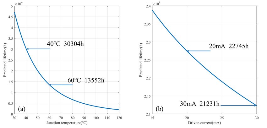
Materials 2018, 11, 817                                                                            2 of 11

for LED products [19,20]. For instance, Qian et al. developed a CSADT method to reduce the reliability
test period from 6000 h to 2000 h for LED luminaires and lamps [21]. Via a boundary curve theory,
they proved that the qualification results obtained from the 6000 h test data under 25 ◦ C and 1500 h
test data under 55 ◦ C are comparable to each other for a majority of LED lighting products. However,
these studies based on CSADT method focused only on single stress and did not build up relationship
between lifetime and accelerated stresses.
      Through the historical investigations on the degradation characteristics of LEDs, the accelerated
loadings could be high temperature [22], high moisture [23], high driving current [24], a combination
of temperature and moisture [25,26] or a combination of temperature with current [27]. Edirisinghe
et al. used a junction temperature based Arrhenius model to determine the lifetime of 1-W HBLEDs
(high-bright light-emitting diodes) [28]. An accelerated aging test for high-power LEDs under different
high-temperature stresses without input current was conducted in [29], which shows that a sufficiently
high-temperature stress effectively shortens the unstable period of the LED chip. Sau Koh et al.
presented an accelerated testing by taking the ambient temperature of 55 ◦ C as the accelerated stress,
combining the exponential decay model and Arrhenius equation by using a two-stage acceleration
theory [30]. Thermal stress is regarded as having the largest influence on the degradation of LED,
and the mentioned papers often set the ambient temperature as the accelerated stress, which, in fact,
should be junction temperature. Furthermore, these studies investigated the acceleration of single
stress but ignored the coupled influences of the current stresses on each other.
      In addition, the operating conditions of multiple-coupled stresses ADT on LEDs are much more
sophisticated than that of single stress. Wang et al. conducted a thermal–electrical stressed accelerated
degradation test on LED-based light bars. In their study, the effect of current was transferred into
junction temperature [31]. An accelerated life test method with temperature and currents is reported
in [32], i.e., the lifetime of the LEDs was extrapolated by first a temperature stress acceleration and
then a current stress acceleration. Besides, three-stage degradation behavior of GaN-based LEDs
under a thermal–electrical dual stress is demonstrated in [33]. These studies revealed the effects of
thermal–electrical dual stress on LED product. However, there is no specific model to describe the
connection between lifetime and thermal–electrical dual stress.
      The successful applications of CSADT models reveal that acceleration method is quite effective
in shorting the duration of testing to obtain data for LED lifetime estimation. The research focus
concentrates on solving the dilemma between accuracy and universality and enhancing the efficiency
of the ADT method. On the other hand, the current CSADT methods are based on the empirical
models, of which the parameters were often obtained by curve fitting from experimental data [34].
These models conclude the relationship between degradation and operation time, ignoring the loading
conditions in the emission profiles [35].
      To deepen the understanding on the relationship between lifetimes of LEDs and their operating
conditions, the degradation rate of LED under constant thermal and electrical stresses is investigated
in this paper. Then, this paper proposes a lifetime prediction model under dual stresses, which
reveals the physical principle of degradation and loading conditions in LEDs. Furthermore, the linear
accumulated damage model was combined with the lifetime model to predict lifetime under emission
profiles of LEDs. With the lifetime model concerning dual stresses, the lifetime prediction based on
junction temperature and driving current becomes more reliable and correct.
      The remainder of this paper is organized as follows: Section 2 establishes the lifetime model
under thermal and electrical stresses, followed by the solution and analysis on model parameters in
Section 3. The applications and case studies are discussed in Section 4. The concluding remarks are
drawn in Section 5.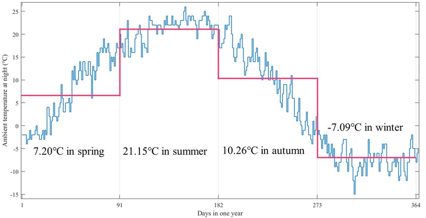
Materials 2018, 11, 817                                                                                  3 of 11

2. The Lifetime Model for LEDs under Thermal and Electrical Stresses
    It is reported in TM-21-11 that the gradual luminous flux degradation follows an exponential
decaying function [7]:
                                            Φ = βe−αt ,                                      (1)

where Φ is the lumen maintenance, β is the pre-factor, and α denotes the decay parameter. For LEDs
products, the failure criterion, denoted as Lp , where p equals 50 or 70 based on different applications,
is defined as the time when lumen maintenance degrades to p%, as given by:

                                             Lp = ln(β/p)/α,                                                (2)

    When applied by thermal and electrical stresses, the degradation rate of the LEDs can be calculated
using Eyring model:                                          !
                                               n         Ea
                                     α = AI exp −              ,                                     (3)
                                                         kTj

where Tj is the absolute temperature in Kelvin; I represents the driving current in LEDs products;
Ea Ea and k denote the activation energy and Boltzmann constant, respectively; and n and A are the
model constants.
     By substituting Equation (3) into Equation (2), the lifetime model under thermal and electrical
stress can be established as:                                       !
                                                     −n         Ea
                                 Lp = ln(β/p)/A · I · exp             ,                          (4)
                                                                kTj

      Next, by using Λ to replace ln( β/p)/A, where τ denotes Lp , Equation (4) can be simplified as:
                                                                  !
                                                   −n         Ea
                                          τ = ΛI        · exp       ,                                       (5)
                                                              kTj

3. Solution and Analysis of the Lifetime Model

3.1. Model Solving
     Equation (6) can be rearranged as Equation (7) by taking natural logarithms on both sides of
the equation.
                                                           Ea
                                    ln τ = ln Λ − n ln I +     ,                              (6)
                                                           kTj
                                                                           Ea
     Letting z = ln τ, x = ln I, y = T1j , γ1 = ln Λ, γ2 = −n, and γ3 =    k ,   the model in Equation (6) can
be transformed into the following formula:

                                            z = γ1 + γ2 x + γ3 y,                                           (7)

     Therefore, the estimation of parameters in the model in Equation (7) can be translated into a
multiple linear regression.
     In the process of solving function, at least three sets of data are needed. Three sets of ( xi , yi , zi )
can be used to estimate Γ = (γ1 , γ2 , γ3 ). The algorithm can be expressed in matrix form:

                                             Z = Γ•(1, X, Y) T ,                                            (8)

where Z = (z1 , z2 , z3 ), X = ( x1 , x2 , x3 ), and Y = (y1 , y2 , y3 ).
    After accelerated degradation testing for LED products, the data of thermal stress, electrical stress
and lumen degradation can be obtained. Furthermore, the lifetime under each stress level can be
Materials 2018, 11, 817 4 of 11
extrapolated using the degradation trajectories of the LED products. These data can be transformed
into parameters in the model algorithm to solve γ1 , γ2 and γ3 .
Furthermore,
Materials thePEER
2018, 11, x FOR lifetime estimation model under thermal–electrical stresses can be expressed
REVIEW 4 ofin
11
Equation (9). !
γ2 γ
γ 3 , ,
τ = Iτ = Iexp
γ
exp T3 ++γ 1γ (9)
1
2
Tj (9)
j
As has been reported in the literature [31], Wang et al. designed five sets of thermal and electrical
As has been reported in the literature [31], Wang et al. designed five sets of thermal and electrical
stress levels to conduct accelerated degradation testing for LED-based light bars, where the junction
stress levels to conduct accelerated degradation testing for LED-based light bars, where the junction
temperature and driving current are designed as accelerated stresses. The first three sets of stresses are
temperature and driving current are designed as accelerated stresses. The first three sets of stresses
selected to solve the lifetime model proposed in this paper, while the remaining two sets of data are
are selected to solve the lifetime model proposed in this paper, while the remaining two sets of data
employed to verify the model.
are employed to verify the model.
The driving currents, ambient temperatures and junction temperatures in each stress level are
The driving currents, ambient temperatures and junction temperatures in each stress level are
listed in Table 1. Meanwhile, Figure 1 demonstrates the average normalized light outputs under
listed in Table 1. Meanwhile, Figure 1 demonstrates the average normalized light outputs under
different stress levels and the fitting degradation trajectories.
different stress levels and the fitting degradation trajectories.
Table 1. Description of stress level conditions.
Table 1. Description of stress level conditions.
Stress Experimental
ExperimentalConditions
Conditions
Stress Level Quantity of Sample Junction
of Sample
Quantity Temperature
Junction T j ( ◦TC)
Temperature j ( °C)
Level (Driving
(Driving Current,
Current, Ambient
Ambient Temperature)
Temperature)
S1 S1 (20 (20
mA,mA,
60 °C)◦
60 C) 15 15 82.482.4
S2 S2 (30 (30
mA,mA, 60 ◦ C)
60 °C) 15 15 93.693.6
S3 (25 mA, 72.5 ◦ C) 15 100.5
S3 (25 mA, 72.5 °C) 15 100.5
S4 (20 mA, 85 ◦ C) 15 107.4
S4 (20 mA, 85 °C)◦ 15 107.4
S5 (30 mA, 85 C) 15 118.6
S5 (30 mA, 85 °C) 15 118.6
Figure 1.
Figure 1. Degradation
Degradation data
data [31]
[31] and
and trajectories
trajectories under
under different
differentstress
stresslevels.
levels.
As shown
As shownin inFigure
Figure1,1,there
thereare
areapparent
apparent discrepancies
discrepancies between
between thethe fitting
fitting curves
curves andanddatadata in
in S3,
S3, S4 and S5 for the early time, while, for longer time, the experimental data fits
S4 and S5 for the early time, while, for longer time, the experimental data fits well with the curves. well with the curves.
Thisphenomenon
This phenomenonmay maybe beexplained
explainedwithwith thethe assumption
assumptionthat that activation
activation energy
energyshift
shift slows
slows down
down the the
luminous flux
luminous fluxdecay,
decay,and
andfor
forlonger
longertime
timethetheactivation
activationenergyenergyturns
turnsback
backtotoits
itsinitial
initialstate.
state.
The expected lifetimes in different stress levels can be obtained using Equations (1) and(1)
The expected lifetimes in different stress levels can be obtained using Equations (2),and (2),
which
which are listed in Table 2. By taking ( x , y
are listed in Table 2. By taking ( x , y , z ) ini Equation
i , z i ) in Equation (8), the parameters are extracted
(8), the parameters are extracted as γ = −2.5774, as γ 1=
i i i 1
γ−2.5774, γ 2 =and
2 = −0.1699
−0.1699 and γ 3 = 4197.9.
γ3 = 4197.9.
Therefore, the lifetime prediction model for the particular test samples in Wang’s study under
thermal and electrical stresses is solved as:
4197.9
τ = I −0.1699 exp − 2.5774 , (10)
T
j Materials 2018, 11, 817 5 of 11
Therefore, the lifetime prediction model for the particular test samples in Wang’s study under
thermal and electrical stresses is solved as:
!
−0.1699 4197.9
τ=I exp − 2.5774 , (10)
Tj
Table 2. Independent variables for model solution.
Stress Level
Item
S1 S2 S3 S4 S5
Expected lifetime (L50 ) 6126.8 h 3987.7 h 3329.5 h 1582.9 h 1023.2 h
Driving current (I) 20 mA 30 mA 25 mA 20 mA 30 mA
Junction temperature (Tj ) 355.33 K 366.75 K 373.65 K 380.55 K 391.75
Predicted lifetime – – – 3038.0 h 1965.2 h
The quantitative effects of driving current and junction temperature on lifetime can be expressed
in Equation (10), with which the lifetime can be predicted under the given thermal–electrical coupling
conditions. In this paper, the expected lifetime comes from the experimental data while the predicted
lifetime is obtained using proposed model. When the junction temperature and driving current in
S4 and S5 are used in Equation (10), the lifetimes are predicted as 3038.0 h and 1965.2 h, respectively.
There is an obvious deviation between the predicted lifetime and the expected lifetime, i.e., 91.9% for
S4 and 92.1% for S5.
Compared with S3, S4 has higher junction temperature and lower driving current, but the expected
lifetime in S4 is much smaller than that in S3, thus it can be deduced that the degradation mechanism
were changed by the high junction temperature which causes dramatic lifetime drop in S4. Therefore,
the lifetime model should be modified to characterize the mechanism variation in the experiment. The
correction factor ε( Tj , I ) is introduced into the lifetime model:
!
−0.1699 4197.9
τ=I exp − 2.5774 + ε( Tj , I ) , (11)
Tj
ε( Tj , I ) is related with the junction temperature and driven current. Besides, when the stress level
is smaller than stress level that changes the degradation mechanism, ε( Tj , I ) = 0. When strong stress
level is exerted to the LEDs products, ε( Tj , I ) can be estimated with a new set of data. Due to insufficient
experimental data, the detailed degradation mechanism shift cannot be further determined in this
paper. The reasons may lie in the effect of high driving current on LED chips, or high temperature on
packaging materials, or the coupling effects of both factors.
With the data in S4, the correction factor is estimated as ε( Tj , I ) = −0.5778, the correction factor
can be explained as a constant to characterize the changed degradation mechanism. Consequently, the
lifetime is predicted with the modified lifetime model in Equation (11) as 1077.8 h with parameters in
S5, which is quite close to the expected lifetime with an error of (1077.8 − 1023.2)/1023.2 = 5.34%.
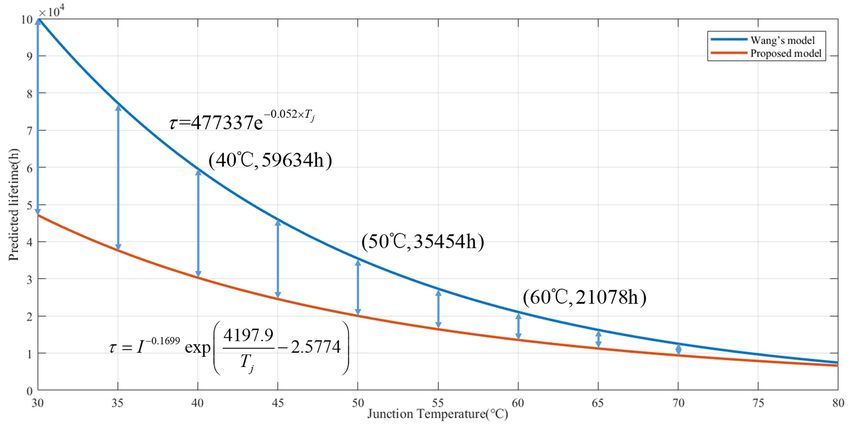
3.2. Compare with Wang’s Model
In addition, compared with the lifetime model in Wang’s study, where the lifetime was given by
τ = 477337e−0.052×Tj , the lifetime predicted by the dual-stress model is lower than that of single-stress
model under the same emission profile, as shown in Figure 2. The phenomenon is due to the ignorance
of the driving current in degenerating the lifetime of LEDs in Wang’s study. Therefore, the driving
current should be considered when modeling with the thermal and electrical stresses ADT data.
In addition, the lifetime gap of the two models becomes smaller as the junction temperature increases;
this tendency is due to the dominant status in the high temperature area of junction temperature.Materials 2018, 11, 817 6 of 11
Materials
Materials2018,
2018,11,
11,xxFOR
FORPEER
PEERREVIEW
REVIEW 66ofof11
11
Figure 2.2.Comparison
Figure2.
Figure ofofWang’s
Comparisonof
Comparison Wang’s model
Wang’smodel [31]
model[31] and
[31]and the
andthe model
themodel proposed
modelproposed ininthis
proposedin this paper.
thispaper.
paper.
3.3. Effects
3.3.Effects
EffectsofofofJunction Temperature
JunctionTemperature
Temperatureand and Driving
andDriving Current
DrivingCurrent on
Currenton Lifetime
onLifetime
Lifetime
3.3. Junction
On the
Onthetheoneone hand,
onehand, when
hand,when LEDs
whenLEDs work
LEDswork under
workunderunderaaaconstant
constant driving
constantdriving current,
drivingcurrent, Equation
current,Equation
Equation(10)(10) follows
(10)follows the
followsthethe
On 1
T1 1/T
formττ τ==
form =γeγe γe , ,which reveals that
thatlifetime decays with
withjunction temperature ininan
anexponential form
formas
j
form T
j j
, which
which reveals
reveals that lifetime
lifetime decays
decays with junction
junction temperature
temperature in an exponential
exponential as
form
shown as shown
in Figure in Figure
3a. Figure3a.
3aFigure
also 3a also
exhibits exhibits
that the that the
sensitivity sensitivity
of lifetime of lifetime
loss is
shown in Figure 3a. Figure 3a also exhibits that the sensitivity of lifetime loss is much more significantmuch loss
moreis much more
significant
significant
atatthe lowat
thelow the low temperature
temperature
temperature are
arethan are
thanthatthatthan that
atatthe
the at the
high
high high temperature
temperature
temperature area. area. Therefore,
area.Therefore,
Therefore, the the attempt
theattempt
attempt to
totolower
lower
junction
lower temperature
junction is
temperature of practical
is of significance
practical in maintaining
significance in longer
maintaining
junction temperature is of practical significance in maintaining longer lifetime. lifetime.
longer lifetime.
Figure 3.3.Expected
Figure3. lifetime
Expectedlifetime decays
lifetimedecays with:
decayswith: junction
with:junction temperature
junctiontemperature (a);
temperature(a); and
(a);and driving
anddriving current
drivingcurrent (b).
current(b).
(b).
Figure Expected
On
Onthetheother
otherhand,
hand,when whenLEDs
LEDsworks
worksunder underaaconstant
constantjunction
junctiontemperature,
temperature,Equation
Equation(10)
(10)
On the other hand, γ 2γwhen LEDs works under a constant junction temperature, Equation (10)
follows
followsthetheform which γγ2 2 isisaanegative
form ττ==βIβI γ2,2,ininwhich negativeconstant
constantandand ββ isispositive.
positive.This
Thisindicates
indicatesthat
that
follows the form τ = βI , in which γ2 is a negative constant and β is positive. This indicates that
lifetime decays
lifetimedecays with
decayswith the
withthe driving
thedriving current
drivingcurrent
currentinininaapower form,
powerform, as
form,as shown
asshown
showninininFigure 3b.
Figure3b.3b.However, dissimilar
However,dissimilar
dissimilar
lifetime a power Figure However,
totothe
the effect
effect of junction
of junction temperature,
temperature, curve of lifetime degradation in Figure 3b is nearly linear
to the effect of junction temperature, curvecurve of lifetime
of lifetime degradation
degradation in Figurein 3b
Figure 3b islinear
is nearly nearly linear
because
because
because the order of the power function is too small. Therefore, the lifetime of LEDs can be
the order of the power function is too small. Therefore, the lifetime of LEDs can be
considerably
considerablyprolonged
prolongedby byreducing
reducingthe
thedriving
drivingcurrent
currentwithin
withinaareasonable
reasonablerange.
range.
The
Thelifetime
lifetimemodel
modeland andcurves
curvesininFigure
Figure33reveal
revealthat
thatlifetime
lifetimedecreases
decreasesmonotonically
monotonicallywith withthe
the
increasing junction temperature and driving current, but the descent rates of the
increasing junction temperature and driving current, but the descent rates of the curves are different. curves are different.Materials 2018, 11, 817 7 of 11
the order of the power function is too small. Therefore, the lifetime of LEDs can be considerably
prolonged by reducing the driving current within a reasonable range.
The lifetime model and curves in Figure 3 reveal that lifetime decreases monotonically with
the increasing junction temperature and driving current, but the descent rates of the curves are
different. Although the driving current has a power law effect, whereas the junction temperature has
an exponential effect, the expected lifetime of LEDs is much more sensitive to the junction temperature
than driving current. For instance, the expected lifetime will increase from 13,552 h to 30,304 h as
junction temperature drops from 60 ◦ C to 40 ◦ C (a decrease of 33.3%), while a decrease of 33.3% in
driving current (from 30 mA to 20 mA) leads a lifetime increase from 21,231 h to 22,745 h.
The result suggests that it is more feasible to maintain a longer lifetime by reducing the junction
temperature. In addition, there are two ways to reduce junction temperature: better cooling condition
and lower driving current. Because a lower driving current in LEDs leads longer lifetime, it is more
practical to reduce driving current when the cooling condition cannot be optimized for the enhance
of lifetime.
4. Applications and Case Study of the Lifetime Model
Generally speaking, an accurate and robust estimation on the expected lifetime of LED products
is vitally important when using them in practical applications, especially under harsh conditions.
However, due to complications from both internal and external environmental stresses, it is not easy to
perform a comprehensive prediction on the expected lifetimes. This section provides a solution based
on Equation (10) on the expected lifetime prediction for LEDs under a complicated emission profile
with any given combinations between varying temperatures and driving currents.
For a given operational condition of ambient temperature and driving current, the corresponding
lifetime can be predicted using the lifetime model. However, in the outdoor application of LEDs, the
ambient temperature and loading conditions often change, causing variation of junction temperature
and driving current. Based on assumption of linear accumulated damage model [36], the consumed
lumen lifetime can be predicted as:
n
t
CL = ∑ i , (12)
τ
i =1 i
where n is the number of stress levels, ti is the accumulated duration at stress ( Tj , I )i , and τi is the
corresponding lifetime. Therefore, the lumen lifetime under varying ambient and loading conditions
is the time when CL reaches 1. Assuming that the duration of ambient conditions is periodic, the total
n
1
lifetime can be calculated by τ = CL ∑ ti .
i =1
Unlike the indoor application, the outdoor application such as street lamp endures variable
ambient temperature at different seasons in one year. The LED lamps works at rated current from
19:00 p.m. to the next day 5:00 a.m., lasting 10 h per day, while the ambient temperature varies with
seasons. Take Beijing as an example: the average ambient temperatures at night from spring to winter
are 7.20 ◦ C, 21.15 ◦ C, 10.26 ◦ C and −7.09 ◦ C respectively, as demonstrated in Figure 4. For the sake
of facilitating calculation, the assumption that a quarter contains 91 days and exclusion of current
fluctuation is reasonable.
Under this circumstance, the number of stress level n is 4, and the accumulated duration at each
stress level ti equals 910 h. Based on the proposed model, the corresponding predicted lumen lifetimes
at each stress level are listed in Table 3.
Based on Formula (12), the consumed life can be calculated as CL = t1/τ1 + t2/τ2 + t3/τ3 + t4/τ4 =
0.1184, thus the prediction of total lumen lifetime under given emission profile is τ = 4t/CL = 30, 735 h.Materials 2018, 11, 817 8 of 11
Table 3. Predicted lumen lifetimes under various emission profiles.
No. Season Accumulated Duration Stress Level (T a , I) Predicted Lifetime (τ)
1 Spring 910 h (7.20 ◦ C,
20 mA) 34,201 h
2 Summer 910 h (21.15 ◦ C, 20 mA) 19,113 h
3 Autumn 910 h (10.26 ◦ C, 20 mA) 29,969 h
4 Winter 910 h (−7.09 ◦ C, 20 mA) 65,702 h
Materials 2018, 11, x FOR PEER REVIEW 8 of 11
Figure 4.
Figure 4. The
The average
average ambient
ambient temperature
temperature at
at night
night every
every day
dayin
inBeijing.
Beijing.
5. Conclusions
5. Conclusions
In this
In thispaper,
paper,the theexpected
expected lifetime
lifetime related
related to lumen
to lumen degradation
degradation of LEDs
of LEDs under under
bothboth thermal
thermal and
and electrical stresses are investigated and predicted using the dual-stress
electrical stresses are investigated and predicted using the dual-stress lifetime model. With the lifetime model. With the
experimental data
experimental data in in [31],
[31], the
the lifetime
lifetime model model was was established
established and and validated,
validated, which which proved
proved the the
availability and effectiveness of the model. The experimental data
availability and effectiveness of the model. The experimental data also exhibit that the degradation also exhibit that the degradation
mechanismwas
mechanism waschanged
changedby bythethe high
high level
level of of acceleration
acceleration stresses,
stresses,butbutthe
the critical
critical value
value ofof stress
stress level
level
wasnot
was notdetermined
determineddue dueto tothe
thelack
lackof of necessary
necessary data. data. AA correction
correction factor
factor was
was introduced
introduced to to enhance
enhance
the accuracy of lifetime prediction under high stress level, with which
the accuracy of lifetime prediction under high stress level, with which the relative error drops from the relative error drops from
92.1% to
92.1% to 5.34%.
5.34%. When
When the the stress
stress level
level is is lower
lower than
than thethe critical
critical value, the correction
value, the factor equals
correction factor equals zero,
zero,
or, other cases, more data are required to determine the
or, other cases, more data are required to determine the new critical stress level. new critical stress level.
In addition,
In addition, the the predicted
predicted lifetime
lifetime is is smaller
smaller withwith the
the dual-stress
dual-stress lifetime
lifetime model
model thanthan that
that with
with
Wang’smodel
Wang’s modeldue dueto tothe
the coupling
coupling effect effect of of driving
driving current
current onon both
both lifetime
lifetime and
and junction
junction temperature.
temperature.
Therefore, it is revealed that driving current is another crucial factor
Therefore, it is revealed that driving current is another crucial factor when predicting lifetime when predicting lifetime and
and
cannot be ignored in modeling with thermal and
cannot be ignored in modeling with thermal and electrical stresses ADT data.electrical stresses ADT data.
The comparison
The comparison betweenbetween the the effects
effects of of junction
junction temperature
temperature and and driving
driving current
current on on lifetime
lifetime
indicates that the lifetime of LEDs is more sensitive to the thermal stress,
indicates that the lifetime of LEDs is more sensitive to the thermal stress, i.e., junction temperature, i.e., junction temperature,
while electrical
while electrical stress
stressalso
alsocauses
causesdepreciation
depreciationin inlifetime.
lifetime. InIn the
the discussion,
discussion, the the lifetime
lifetime decays
decays with
with
junction temperature in an exponential form, a slight fluctuation in
junction temperature in an exponential form, a slight fluctuation in junction temperature will cause junction temperature will cause
great drop
great drop in in lifetime.
lifetime. Therefore,
Therefore, more more efforts
efforts should
should be be paid
paid ononreducing
reducing the thejunction
junction temperature
temperature
of LEDs.
of LEDs.
Furthermore, aa method
Furthermore, method that that combines
combines linear linear accumulated
accumulated damagedamage theory
theory with with the
the dual-stress
dual-stress
lifetime model is proposed to predict lifetime of LEDs product under variable stresses. case
lifetime model is proposed to predict lifetime of LEDs product under variable stresses. The Thestudy
case
makes it unequivocal that the lifetime model can be successfully applied
study makes it unequivocal that the lifetime model can be successfully applied to the circumstances of to the circumstances of
constant and variable
constant and variable stresses. stresses.
However, this paper considers only the luminous depreciation in LED for lifetime prediction,
and the model cannot characterize other failure models such as color shift and catastrophic failure.
Besides, the statistic properties of life data from accelerated degradation testing were not considered
during the model solving. The lifetime prediction model based on color shift and exploration for
advanced statistical methods will be conducted in the prospective work.Materials 2018, 11, 817 9 of 11
However, this paper considers only the luminous depreciation in LED for lifetime prediction, and
the model cannot characterize other failure models such as color shift and catastrophic failure. Besides,
the statistic properties of life data from accelerated degradation testing were not considered during
the model solving. The lifetime prediction model based on color shift and exploration for advanced
statistical methods will be conducted in the prospective work.
Author Contributions: Conceptualization, X.Y. and C.Q.; Methodology, software and validation, X.Y. and
D.Y.; Investigation, B.S.; Resources, Z.W., Y.R.; Data Curation, Q.F.; Writing-Original Draft Preparation, X.Y.;
Writing-Review & Editing, B.S. and C.Q.; Visualization, X.Y.; Supervision, Z.W.; Project Administration, Y.R.;
Funding Acquisition, B.S.
Funding: This research was funded by the National Natural Science Foundation (NFSC) of China (No. 61673037).
Acknowledgments: The founding sponsors had no role in the design of the study; in the collection, analyses, or
interpretation of data; in the writing of the manuscript, and in the decision to publish the results.
Conflicts of Interest: The authors declare no conflict of interest.
Nomenclature
Φ Lumen maintenance
β Pre-factor of LED’s depreciation
α Degradation rate of LEDs
Lp Failure criterion of LEDs
Tj Junction temperature in LEDs
I Driving current
Ea LED’s activation energy
k Boltzmann constant
n Model constant
A Model constant
References
1. Van Driel, W.D.; Fan, X.J. Solid State Lighting Reliability: Components to Systems; Springer: New York, NY, USA, 2012.
2. Chang, M.H.; Das, D.; Varde, P.V.; Pecht, M. Light emitting diodes reliability review. Microelectron. Reliab.
2012, 52, 762–782. [CrossRef]
3. Qian, C.; Fan, J.J.; Fang, J.; Yu, C.; Ren, Y.; Fan, X.J.; Zhang, G.Q. Photometric and colorimetric assessment of
LED chip scale packages by using a step-stress accelerated degradation test (SSADT) method. Materials 2017,
10, 1181. [CrossRef] [PubMed]
4. Fan, J.J.; Qian, C.; Yung, K.C.; Fan, X.J.; Zhang, G.Q.; Pecht, M. Optimal design of life testing for
high-brightness white LEDs using the six sigma DMAIC approach. IEEE Trans. Device Mater. Reliab.
2015, 15, 576–587. [CrossRef]
5. Sun, B.; Jiang, X.P.; Yung, K.-C.; Fan, J.J.; Pecht, M. A review of prognostics techniques for high-power white
LEDs. IEEE Trans. Power Electron. 2017, 32, 6338–6362. [CrossRef]
6. IES-LM-80-08 Approved Method for Lumen Maintenance Testing of LED Light Source; Illuminating Engineering
Society: New York, NY, USA, 2008.
7. IES-TM-21-11 Projecting Long Term Lumen Maintenance of LED Light Sources; Illuminating Engineering Society:
New York, NY, USA, 2011.
8. Huang, J.L.; Golubović, D.S.; Koh, S.; Yang, D.G.; Li, X.P.; Fan, X.J.; Zhang, G.Q. Degradation modeling
of mid-power white-light LEDs by using Wiener process. Opt. Express 2015, 23, A966–A978. [CrossRef]
[PubMed]
9. Fan, J.J.; Yung, K.C.; Pecht, M. Lifetime estimation of high-power white LED using degradation-data-driven
method. IEEE Trans. Device Mater. Reliab. 2012, 12, 470–477. [CrossRef]
10. Tao, X.H.; Hui, S.Y.R. Dynamic photoelectrothermal theory for light-emitting diode systems. IEEE Trans.
Ind. Electron. 2012, 59, 1751–1759. [CrossRef]Materials 2018, 11, 817 10 of 11
11. Hui, S.Y.R.; Chen, H.; Tao, X.H. An Extended photoelectrothermal theory for LED systems: A tutorial from
device characteristic to system design for general lighting. IEEE Trans. Power Electron. 2012, 27, 4571–4583.
[CrossRef]
12. Hui, S.Y.R.; Qin, Y.X. A General photo-electro-thermal theory for light emitting diode (LED) systems.
IEEE Trans. Power Electron. 2009, 24, 1967–1976. [CrossRef]
13. Watzke, S.; Altieri-Weimar, P. Degradation of silicone in white LEDs during device operation: A finite
element approach to product reliability prediction. Microelectron. Reliab. 2015, 55, 733–737. [CrossRef]
14. Fischer, H.R.; Semprimoschnig, C.; Mooney, C.; Rohr, T.; van Eck, E.R.H.; Verkuijlen, M.H.W. Degradation
mechanism of silicone glues under UV irradiation and options for designing materials with increased
stability. Polym. Degrad. Stabil. 2013, 98, 720–726. [CrossRef]
15. Sun, B.; Fan, X.J.; Ye, H.Y.; Fan, J.J.; Qian, C.; Van Driel, W.D.; Zhang, G.Q. A novel lifetime prediction for
integrated LED lamps by electronic-thermal simulation. Reliab. Eng. Syst. Saf. 2017, 163, 14–21. [CrossRef]
16. Huang, J.; Golubovic, D.S.; Koh, S.; Yang, D.; Li, X.; Fan, X.; Zhang, G.Q. Lumen degradation modeling
of white-light LEDs in step stress accelerated degradation test. Reliab. Eng. Syst. Saf. 2016, 154, 152–159.
[CrossRef]
17. Han, D. Time and cost constrained optimal designs of constant-stress and step-stress accelerated life tests.
Reliab. Eng. Syst. Saf. 2015, 140, 1–14. [CrossRef]
18. Benavides, E.M. Reliability Model for step-stress and variable-stress situations. IEEE Trans. Reliab. 2011, 60,
219–233. [CrossRef]
19. Hamon, B.; van Driel, W.D. LED degradation: From component to system. Microelectron. Reliab. 2016, 64,
599–604. [CrossRef]
20. Mehr, M.Y.; Van Driel, W.D.; Zhang, G.Q. Reliability and lifetime prediction of remote phosphor plates in
solid-state lighting applications using accelerated degradation testing. J. Electron. Mater. 2016, 45, 444–452.
[CrossRef]
21. Qian, C.; Fan, X.J.; Fan, J.J.; Yuan, C.A.; Zhang, G.Q. An accelerated test method of luminous flux depreciation
for LED luminaires and lamps. Reliab. Eng. Syst. Saf. 2016, 147, 84–92. [CrossRef]
22. Trevisanello, L.; Meneghini, M.; Mura, G.; Vanzi, M.; Pavesi, M.; Meneghesso, G.; Zanoni, E. Accelerated life
test of high brightness light emitting diodes. IEEE Trans. Device Mater. Reliab. 2008, 8, 304–311. [CrossRef]
23. Luo, X.B.; Wu, B.L.; Liu, S. Effects of moist environments on LED module reliability. IEEE Trans. Device
Mater. Reliab. 2010, 10, 182–186. [CrossRef]
24. Yanagisawa, T.; Kojima, T. Long-term accelerated current operation of white light-emitting diodes. J. Lumines.
2005, 114, 39–42. [CrossRef]
25. Huang, J.; Golubović, D.S.; Koh, S.; Yang, D.; Li, X.; Fan, X.J.; Zhang, G.Q. Rapid degradation of mid-power
white-light LEDs in saturated moisture conditions. IEEE Trans. Device Mater. Reliab. 2015, 15, 478–485.
[CrossRef]
26. Huang, J.; Golubović, D.S.; Koh, S.; Yang, D.; Li, X.; Fan, X.J.; Zhang, G.Q. Degradation mechanisms of
mid-power white-light LEDs under high-temperature–humidity conditions. IEEE Trans. Device Mater. Reliab.
2015, 15, 220–228. [CrossRef]
27. Vázquez, M.; Núñez, N.; Nogueira, E.; Borreguero, A. Degradation of AlInGaP red LEDs under drive current
and temperature accelerated life tests. Microelectron. Reliab. 2010, 50, 1559–1562. [CrossRef]
28. Edirisinghe, M.; Rathnayake, P. Arrhenius accelerated life test for luminary life of high bright light emitting
diodes. Int. Lett. Chem. Phys. Astron. 2015, 49, 48–59. [CrossRef]
29. Yang, Y.H.; Su, Y.F.; Chiang, K.N. Acceleration factor analysis of aging test on gallium nitride (GaN)-based
high power light-emitting diode (LED). In Proceedings of the Thermal and Thermomechanical Phenomena
in Electronic Systems (ITherm), Orlando, FL, USA, 27–30 May 2014.
30. Koh, S.; Yuan, C.; Sun, B.; Li, B.; Fan, X.J.; Zhang, G.Q. Product level accelerated lifetime test for indoor LED
luminaires. In Proceedings of the Thermal, Mechanical and Multi-Physics Simulation and Experiments in
Microelectronics and Microsystems (EuroSimE), Wroclaw, Poland, 14–17 April 2013.
31. Wang, F.K.; Chu, T.P. Lifetime predictions of LED-based light bars by accelerated degradation test.
Microelectron. Reliab. 2012, 52, 1332–1336. [CrossRef]
32. Nogueira, E.; Mateos, J. Accelerated life testing LEDs on temperature and current. In Proceedings of the
Electron Devices (CDE), Palma de Mallorca, Spain, 8–11 February 2011.Materials 2018, 11, 817 11 of 11
33. Liu, L.; Ling, M.; Yang, J.; Xiong, W.; Jia, W.; Wang, G. Efficiency degradation behaviors of current/thermal
co-stressed GaN-based blue light emitting diodes with vertical-structure. J. Appl. Phys. 2012, 111, 093110.
[CrossRef]
34. Huang, S.D.; Zhou, L.; Cao, G.Z.; Liu, H.Y.; Hu, Y.M.; Jing, G.; Cao, M.G.; Xiao, W.P.; Liu, Y. A novel
multiple-stress-based predictive model of LEDs for rapid lifetime estimation. Microelectron. Reliab. 2017, 78,
46–52. [CrossRef]
35. Qu, X.; Wang, H.; Zhan, X.; Blaabjerg, F.; Chung, H.S.H. A lifetime prediction method for LEDs considering
real mission profiles. IEEE Trans. Power Electron. 2017, 32, 8718–8727. [CrossRef]
36. Miner, M. Cumulative damage in fatigue. J. Appl. Mech. 1945, 12, A159–A164.
© 2018 by the authors. Licensee MDPI, Basel, Switzerland. This article is an open access
article distributed under the terms and conditions of the Creative Commons Attribution
(CC BY) license (http://creativecommons.org/licenses/by/4.0/).You can also read