Magnetodisc modelling in Jupiter's magnetosphere using Juno magnetic field data and the paraboloid magnetic field model - ann-geophys.net
←
→
Page content transcription
If your browser does not render page correctly, please read the page content below

Ann. Geophys., 37, 101–109, 2019
https://doi.org/10.5194/angeo-37-101-2019
© Author(s) 2019. This work is distributed under
the Creative Commons Attribution 4.0 License.

Magnetodisc modelling in Jupiter’s magnetosphere using Juno
magnetic field data and the paraboloid magnetic field model
Ivan A. Pensionerov1 , Elena S. Belenkaya1 , Stanley W. H. Cowley2 , Igor I. Alexeev1 , Vladimir V. Kalegaev1 , and
David A. Parunakian1
1 Federal State Budget Educational Institution of Higher Education M.V. Lomonosov Moscow State University, Skobeltsyn
Institute of Nuclear Physics (SINP MSU), 1(2), Leninskie gory, GSP-1, Moscow 119991, Russian Federation
2 Department of Physics & Astronomy, University of Leicester, Leicester LE1 7RH, UK

Correspondence: Ivan A. Pensionerov (pensionerov@gmail.com)

Received: 6 July 2018 – Discussion started: 12 July 2018
Revised: 18 January 2019 – Accepted: 27 January 2019 – Published: 5 February 2019

Abstract. One of the main features of Jupiter’s magneto-        a steady-state MHD magnetodisc model in which both cen-
sphere is its equatorial magnetodisc, which significantly in-   trifugal and plasma pressure (assumed isotropic) forces were
creases the field strength and size of the magnetosphere.       included, and by Nichols (2011), who incorporated a self-
Analysis of Juno measurements of the magnetic field during      consistent plasma angular velocity model. Nichols et al.
the first 10 orbits covering the dawn to pre-dawn sector of     (2015) have also included the effects of plasma pressure
the magnetosphere (∼03:30–06:00 local time) has allowed         anisotropy, as observed in Voyager and Galileo particle mea-
us to determine optimal parameters of the magnetodisc using     surements, which redistributes the azimuthal currents in the
the paraboloid magnetospheric magnetic field model, which       magnetodisc, changing its thickness.
employs analytic expressions for the magnetospheric current        Here we model the magnetic field observations during
systems. Specifically, within the model we determine the size   Juno’s first 10 orbits for which both inbound and outbound
of the Jovian magnetodisc and the magnetic field strength at    passes are presently available, corresponding to perijoves
its outer edge.                                                 (PJs) 0 to 9, using the semi-empirical global paraboloid Jo-
                                                                vian magnetospheric magnetic field model derived by Alex-
                                                                eev and Belenkaya (2005). We focus on the middle magne-
                                                                tosphere, observed on these orbits in the dawn to pre-dawn
1   Introduction                                                sector of the magnetosphere (∼03:30–06:00 local time, LT),
                                                                for which the magnetodisc provides the main contribution to
In this paper we consider magnetic field measurements made      the magnetospheric magnetic field. In the model, in which
by the Juno spacecraft in Jupiter’s magnetosphere, paying       the field contributions are calculated using parameterised an-
particular attention to the middle magnetosphere measure-       alytic equations, the magnetodisc is described by a simple
ments where Jupiter’s magnetodisc field plays a major role.     thin plane disc lying in the planetary magnetic equatorial
The structure and properties of the Jovian magnetodisc have     plane. We thus search the paraboloid model magnetodisc in-
been described in many papers, starting from the first space-   put parameters to determine the best fit to the Juno measure-
craft flybys of Jupiter, discussed for example by Barbosa       ments. We note that the magnetodisc may be regarded as the
et al. (1979) and references therein. In particular, the em-    most important source of magnetic field in Jupiter’s magne-
pirical magnetodisc model presented by Connerney et al.         tosphere, with a magnetic moment in the model derived by
(1981), derived from Voyager-1 and -2 and Pioneer-10 ob-        Alexeev and Belenkaya (2005) using Ulysses inbound data,
servations, has been employed as a basis in numerous sub-       for example, which is 2.6 times the planetary dipole moment.
sequent studies, including predictions for the Juno mission     Consequently, the magnetodisc plays a major role in deter-
by Cowley et al. (2008, 2017). Detailed physical models         mining the size of the system in its interaction with the solar
have also been constructed by Caudal (1986), who derived

Published by Copernicus Publications on behalf of the European Geosciences Union.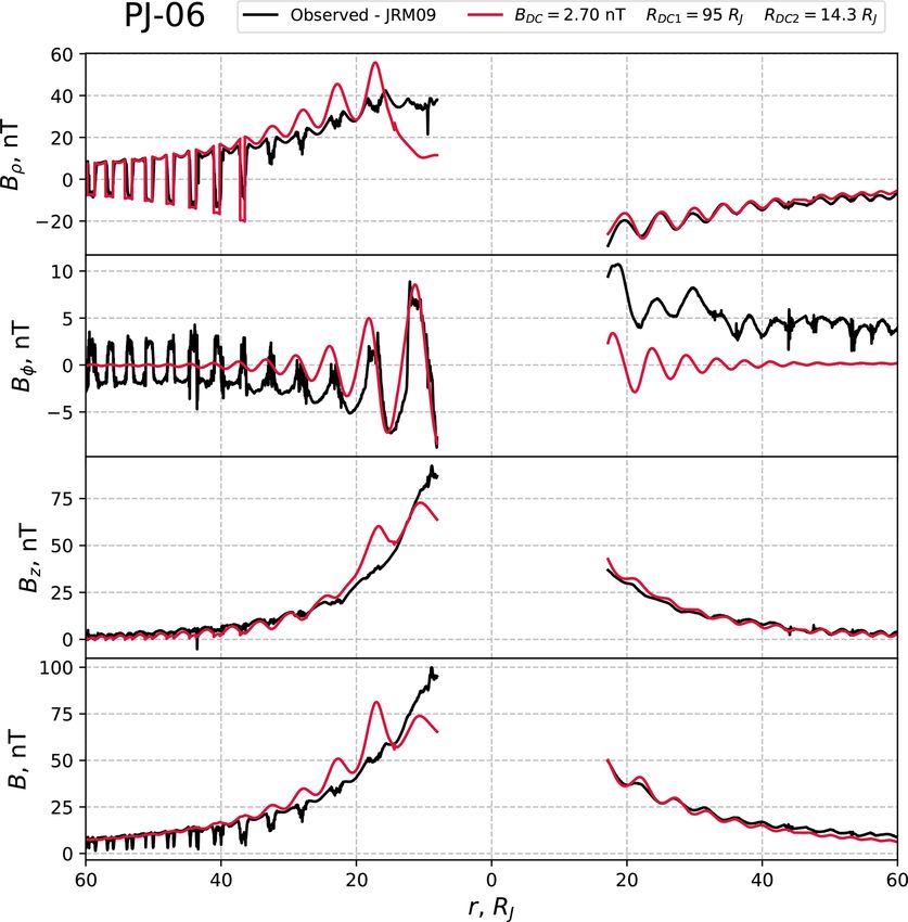
102                 I. A. Pensionerov et al.: Analysis of Juno magnetic field data using paraboloid magnetospheric model

                                                                      tance to the subsolar magnetopause, where y = 0 and z = 0.
                                                                      The magnetospheric magnetic field, B m , is then the sum of
                                                                      the fields created by all these current systems:

                                                                      B m = B i (9) + B TS (9, Rss , R2 , Bt )
                                                                          + B MD (9, BDC , RDC1 , RDC2 ) + B si (9, Rss )
                                                                          + B sMD (9, Rss , BDC , RDC1 , RDC2 ) + kB IMF ,          (2)

                                                                      where 9 is Jupiter’s dipole tilt angle relative to the z axis.
                                                                      The magnetodisc is approximated as a thin disc with outer
                                                                      and inner radii RDC1 and RDC2 , respectively. BDC is the mag-
                                                                      netodisc field at the outer boundary, while the azimuthal cur-
                                                                      rents in the disc are assumed to decrease as r −2 . R2 is the
                                                                      distance to the inner edge of the tail current sheet, and Bt is
                                                                      the tail current magnetic field there. The magnetospheric cur-
                                                                      rent systems are thus described by nine input parameters, de-
                                                                      termining the physical size of the current systems, and their
                                                                      magnetic field (current) strength (9, Rss , R2 , RDC1 , RDC2 ,
                                                                      Bt , BDC , k, B IMF ). In Fig. 1 we show sketches illustrating the
                                                                      parameters of the model. On the left we show a view in the
                                                                      magnetospheric equatorial plane, where we note that in the
Figure 1. In (a) we show a schematic of Jupiter’s magnetosphere       physical system, the overlapping model magnetodisc and tail
in the magnetic equatorial plane, showing various parameters of the   current sheets merge together on the nightside. On the right
paraboloid model. In (b) we show the definition of the planetary      we show the planetary magnetic dipole axis at angle 9 in the
magnetic dipole angle 9 in the JSM system, where XJSM points          JSM system. As shown by Alexeev and Belenkaya (2005),
towards the Sun and the planetary dipole is contained in the XJSM –   the magnetic moment of the model current disc is given by
ZJSM plane.

                                                                                BDC 3               RDC2
                                                                      MMD =           R        1−           .                        (3)
                                                                                  2 DC1             RDC1
wind and is thus an appropriate focus of a study using Juno
magnetic field data.                                                     Alexeev and Belenkaya (2005) and Belenkaya (2004) de-
                                                                      termined model parameters which approximated the mag-
2   The Jupiter paraboloid model                                      netic field along the Ulysses inbound trajectory rather
                                                                      well. These parameters are Rss = 100 RJ , R2 = 65 RJ ,
The paraboloid magnetospheric magnetic field model was                Bt = −2.5 nT, RDC1 = 92 RJ , RDC2 = 18.4 RJ , and BDC =
developed for Jupiter by Alexeev and Belenkaya (2005),                2.5 nT. This set of parameters is used in the present paper as
based on the terrestrial paraboloid model of Alexeev (1986)           a starting point for fitting parameters to the Juno data. The
and Alexeev et al. (1993). It contains the internal plane-            dipole tilt angle 9 changes during the observations and is
tary field, B i , calculated from the full order-4 VIP4 model         calculated as a function of time in the paraboloid model.
of Connerney et al. (1998); the magnetodisc field, B MD ;
the field of the magnetopause shielding currents, B si and
B sMD , which screen the planetary and magnetodisc fields, re-        3   Magnetic field calculations for the first 10 Juno orbits
spectively; the field of the magnetotail current system, B TS ;
and the penetrating part of the interplanetary magnetic field         As indicated above, field calculations have been made us-
(IMF), kB IMF , where k is the IMF penetration coefficient.           ing the paraboloid model for comparison with the data from
The magnetopause is described by a paraboloid of revolution           the first 10 Juno orbits for which data are presently avail-
in Jovian solar magnetospheric (JSM) coordinates with the             able for study. The orbits were closely polar, with large ec-
origin at Jupiter’s centre:                                           centricity, and with apoapsis initially located south of the
                                                                      equator in the dawn magnetosphere (e.g. Connerney et al.,
 x       y 2 + z2                                                     2017). In Fig. 2 we show the perijove 1 trajectory versus time
    = 1−      2
                  ,                                            (1)    (in day of year (DOY) 2016) in JSM Cartesian coordinates,
Rss        2Rss
                                                                      specifically showing
                                                                                      p     the cylindrical and spherical radial dis-
where x is directed towards the Sun, the x–z plane contains           tances ρJSM = x 2 + y 2 and r, ZJSM , and the LT. The ver-
the planet’s magnetic moment, and y completes the right-              tical dashed line shows the time of periapsis. On later orbits
hand orthogonal set pointing towards dusk. Rss is the dis-            apoapsis moved towards the nightside, reaching 03:30 LT by

Ann. Geophys., 37, 101–109, 2019                                                               www.ann-geophys.net/37/101/2019/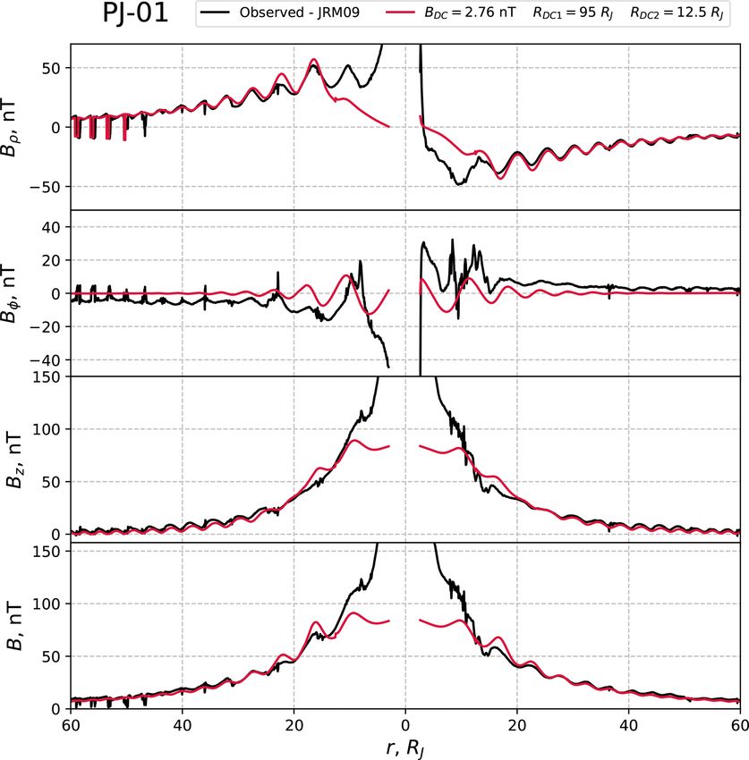
I. A. Pensionerov et al.: Analysis of Juno magnetic field data using paraboloid magnetospheric model                              103

                                                                    the contributions to the magnetospheric field from the mag-
                                                                    netopause and tail current systems (which are oppositely di-
                                                                    rected near the dawn–dusk meridian) are negligible com-
                                                                    pared with the magnetodisc field, being less than 10 % for
                                                                    perijove 1 and less than 16 % for perijove 9, and may thus be
                                                                    treated approximately inside this distance. For related rea-
                                                                    sons we also neglect the penetrating IMF term in Eq. (2),
                                                                    which is unknown when Juno is inside the magnetosphere,
                                                                    highly variable in direction with time, and typically of mag-
                                                                    nitude ∼ 0.1–1 nT (Nichols et al., 2006, 2017). This field too,
                                                                    with penetration coefficient k < 1, is therefore similarly neg-
                                                                    ligible in the r < 60 RJ middle magnetosphere studied here.
                                                                       As a consequence of these considerations, here we employ
                                                                    the JRM09 model of the internal field and fit only the magne-
                                                                    todisc parameters to the middle magnetosphere data. For the
                                                                    small fields contributed by the magnetopause and tail current
                                                                    systems in this regime, we simply use the Ulysses parameters
                                                                    from Alexeev and Belenkaya (2005) and Belenkaya (2004)
                                                                    as sufficient approximations, i.e. Rss = 100 RJ , R2 = 65 RJ ,
                                                                    and Bt = −2.5 nT. However, use of the Ulysses magnetodisc
                                                                    parameters is found to lead, for example, to a systematic un-
                                                                    derestimation of the field along the perijove 1 trajectory, and
                                                                    thus needs to be modified. Thus only three parameters, RDC1 ,
                                                                    RDC2 , and BDC , need to be fitted.
Figure 2. Juno perijove 1 trajectory in JSM Cartesian coordinates      To optimise the model we choose the approach of min-
plotted versus time in DOY 2016, where the vertical dashed line     imising function S given by
shows the time of periapsis.                                                                 v
                                                                                                                    (n) 2
                                                                                             u
                                                                                                          (n)
                                                                                                    N B       − B obs
                                                                                             u
                                                                                             u1 X         mod
                                                                    S(BDC , RDC1 , RDC2 ) = u                             ,      (4)
                                                                                                               (n) 2
                                                                                             tN
perijove 9, and also rotated further into the Southern Hemi-                                       n=1       B obs
sphere.
   In this paper we confine our attention to the middle magne-               (n)
tosphere, where, as we now show, the magnetic field is domi-        where B mod is the modelled field vector due to the current
                                                                                 (n)
nated by the magnetodisc and the planetary field. In the outer      systems, B obs is the observed residual field following sub-
magnetosphere the field becomes strongly influenced by ex-          traction of the JRM09 internal field model, n is the index
ternal conditions in the solar wind, and although in some cir-      number of the data point along the trajectory, and the to-
cumstances these can be reasonably well predicted by MHD            tal number of points is N. S represents a root-mean-square
models initialised using data obtained near Earth’s orbit (e.g.     relative deviation of the modelled magnetic field from the
Tao et al., 2005; Zieger and Hansen, 2008), they will typi-         observed field vectors. We used a relative deviation instead
cally vary strongly on the timescale of the Juno orbit (Fig. 2),    of an absolute value to equalise the influence of all the data
and with them too the outer magnetospheric field. In Figs. 3        points, noting that the magnetic field varies in magnitude sig-
and 4, for example, we show the magnitudes of the modelled          nificantly along the part of the trajectory examined here (see
field from different sources along the inbound (a) and out-         Figs. 3 and 4). Use of the absolute deviation gives good re-
bound (b) passes of perijoves 1 and 9, respectively, plotted        sults in the region closer to the planet where the field magni-
versus radial distance. The red lines in these figures show the     tude is greater, but a poorer fit in other parts of the trajectory.
internal JRM09 (“Juno reference model through perijove 9”)             With regard to the choice of interval employed to min-
planetary field derived by Connerney et al. (2018), which em-       imise S, we note that use of data from the innermost region
ploys the well-determined degree and order 10 coefficients          is not optimal. The JRM09 internal planetary field model dif-
from an overall degree 20 spherical harmonic fit to the data        fers from observations at periapsis (1.06 RJ ) by 0.3 × 10⁵ nT
(plus disc model field) from the first nine Juno orbits. The        (Connerney et al., 2018), which is reasonable accuracy for
black lines show the field of the various magnetospheric cur-       describing an observed field of magnitude ∼ 8 × 10⁵ nT, but
rent systems in the paraboloid model as marked, where the           does not allow us to distinguish the magnetodisc field of or-
model parameters employed are those derived from Ulysses            der 100 nT on this background. We thus restricted the inner
inbound data by Alexeev and Belenkaya (2005), as outlined           border of the interval to consider r > 5 RJ only. However, on
in Sect. 2. It can be seen from Figs. 3 and 4 that for r < 60 RJ    most passes examined here, the inner radial limit is set in-

www.ann-geophys.net/37/101/2019/                                                               Ann. Geophys., 37, 101–109, 2019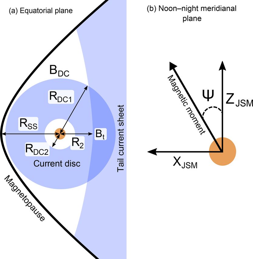
104                  I. A. Pensionerov et al.: Analysis of Juno magnetic field data using paraboloid magnetospheric model

Figure 3. Magnitude of the model magnetic fields for the Juno perijove 1 inbound (a) and outbound (b) passes, due to the internal planetary
field (JRM09, in red), and the various model magnetospheric currents as marked (magnetopause, tail, and magnetodisc, in black).

Figure 4. As for Fig. 3, but for perijove 9.

stead at somewhat larger radii by the data that are presently           parison with the normal runs. Specifically, we stopped the
available for study. A further limitation on the region of cal-         calculation when dS < 0.1S, where dS is the change of func-
culation of S in the outer magnetosphere arises from the fact           tion S in the algorithm step. We then estimated the error as
that the paraboloid model does not display regions of low               (Pmax –Pmin )/2, where Pmax and Pmin are the maximum and
field strength during intersections with the magnetodisc, as            minimum parameter values obtained in these runs. For all
is observed in the field at larger distances, due to the use of         the Juno fits we found that the best-fit outer disc radius RDC1
the infinitely thin disc approximation (see Sect. 4). It is thus        was the maximum value of 95 RJ allowed in the fitting pro-
necessary to avoid these regions by excluding parts of the              cess, set by requiring that the disc radius should be less than
trajectory where the spacecraft is closer than 4 RJ from the            the subsolar magnetopause radius (100 RJ ) by a few RJ . This
magnetic equator.                                                       indicates that the current density in the model disc, varying
   We thus minimise S in the inbound and outbound radial                as r −2 , decreases somewhat too quickly with distance. The
ranges between Rmin and Rmax on each pass to determine the              values of the inner disc radius RDC2 lie between 12.5 and
best-fit magnetodisc parameters. The minimisation was un-               18.7 RJ , usually smaller than the value of 18.4 RJ , derived
dertaken using the trust region reflective procedure (Branch            from the Ulysses data, while the field strength parameter BDC
et al., 1999). The best-fit values are given, together with the         varies between 2.6 and 3.1 nT, larger than the Ulysses value
estimated error values and the radial ranges employed, in Ta-           of 2.5 nT.
ble 1, where we also compare with the values derived by                    In Figs. 5 and 6 we provide comparisons of the observed
Alexeev and Belenkaya (2005) from Ulysses inbound data.                 (black) and modelled (red) residual fields for Juno perijoves 1
We estimated parameter errors by choosing several different             and 6, respectively, from which the JRM09 planetary field
starting points for the algorithm in parameter space and run-           has been subtracted. Specifically we show the JSM cylindri-
ning it with a more generous termination condition in com-              cal field components together with the residual field magni-

Ann. Geophys., 37, 101–109, 2019                                                                 www.ann-geophys.net/37/101/2019/
I. A. Pensionerov et al.: Analysis of Juno magnetic field data using paraboloid magnetospheric model                                         105

Table 1. Magnetodisc parameters derived for the Ulysses inbound pass and the first 10 Juno orbits, together with the estimated errors and the
minimum inbound and outbound radial distances available in the Juno passes.

                                           BDC (nT)     RDC2 (RJ )     RDC1 (RJ )      Rmin (RJ ),      Rmin (RJ ),
                                                                                        inbound         outbound
                             Ulysses            2.50           18.4             92
                             PJ-00       2.58 ± 0.10     18.7 ± 2.8             95    not available        31.5
                             PJ-01       2.76 ± 0.12     12.5 ± 1.8             95         5.0              5.0
                             PJ-02       2.61 ± 0.10     13.6 ± 2.3             95        13.3         not available
                             PJ-03       2.79 ± 0.10     14.5 ± 1.5             95        16.5              8.9
                             PJ-04       2.65 ± 0.07     15.2 ± 1.2             95        13.7             12.3
                             PJ-05       2.59 ± 0.15     14.6 ± 2.5             95        10.6             10.5
                             PJ-06       2.70 ± 0.08     14.3 ± 1.2             95         8.0             17.2
                             PJ-07       3.01 ± 0.09     15.5 ± 2.0             95        21.9             19.7
                             PJ-08       3.07 ± 0.09     15.8 ± 1.9             95        19.5             19.5
                             PJ-09       3.06 ± 0.11     13.6 ± 1.5             95        17.0              8.3

Figure 5. Observed (black) and modelled (red) residual fields in JSM cylindrical components, together with the residual field magnitude, for
Juno perijove 1. The residual field is the observed field with the JRM09 internal field subtracted. The fields are plotted versus spherical radial
distance with inbound data shown on the left and outbound data on the right. The same model field is used for both.

tude plotted versus radial distance, where the same model                  accordance with the observations for the Bρ and Bz compo-
applies to both inbound (left side) and outbound (right side)              nents, while the Bφ component is not adequately described,
data. As can be seen, the fitted models are generally in good              because the model does not include radial currents in the

www.ann-geophys.net/37/101/2019/                                                                        Ann. Geophys., 37, 101–109, 2019
106 I. A. Pensionerov et al.: Analysis of Juno magnetic field data using paraboloid magnetospheric model
Figure 6. As for Fig. 5, but for perijove 6.
magnetodisc and their closure current via the ionosphere. It spectively. The azimuthal current in the disc is taken to vary
is also seen in Fig. 5 that the field magnitude is underesti- as I0 /ρ, where ρ is the perpendicular distance from the plan-
mated inside of ∼ 10 RJ , again probably related to the too- etary dipole magnetic axis. We optimised this model for Juno
steep radial dependence of the azimuthal current. As the dis- perijove 1 using the same method as outlined above, to find
tance from Jupiter decreases, a sharp increase in the residual best-fit parameters I0 = 21 × 106 ARJ−1 (µ0 I0 /2 ≈ 185 nT),
field is observed in the inner region to > 100 nT, while the R0 = 6 RJ , and R1 = 67 RJ . Figure 7 shows a comparison of
model field plateaus at several tens of nanoteslas (nT). At the the observed residual fields (black) with the best-fit Conner-
closest distances from the planet the increase is probably due ney et al. model (blue) in a similar format to Figs. 5 and 6,
to inaccuracy of the JRM09 model of the internal field, not- where we also show the best-fit paraboloid model (red) from
ing that the model represents only the degree and order 10 Fig. 5. One important difference between the model results is
terms from an overall degree 20 fit (Connerney et al., 2018). the fact that the Connerney et al. (1981) model reflects well
the observed periodic sharp drops of magnetic field strength
during spacecraft intersections with the disc. The magne-
4 Approaches for future improvement of the Jupiter todisc radial magnetic field component reverses sign above
paraboloid model and below the disc, and at its centre becomes equal to zero.
As indicated in Sect. 3, the paraboloid model with an in-
We first compare the fits derived here with those obtained finitely thin disc certainly cannot reproduce this feature and
using the magnetodisc model derived by Connerney et al. should thus be improved by use of a disc current of finite
(1981) from Voyager-1 and -2 and Pioneer-10 field data, but thickness. The Connerney et al. model demonstrates reason-
now fitted to Juno perijove 1 data. In this model the current able coincidence with observations near Jupiter, but at greater
flows in a planet-centred annular disc of full thickness 5 RJ , distances overestimates the magnetic field strength, which in-
with inner (R0 ) and outer (R1 ) radii at 5 and ∼ 50 RJ , re-
Ann. Geophys., 37, 101–109, 2019 www.ann-geophys.net/37/101/2019/I. A. Pensionerov et al.: Analysis of Juno magnetic field data using paraboloid magnetospheric model 107
Figure 7. Comparison of the observed residual field (black) and best-fit Connerney et al. (1981) magnetodisc model field (blue) in a similar
format to Fig. 5. We also show the best-fit paraboloid model (red) as in Fig. 5.
dicates that at these distances the current density variation as 5 Discussion and conclusions
ρ −1 is too slow.
As indicated above, neither of the magnetodisc models
considered here describe the azimuthal field well at medium As shown in Figs. 3 and 4, in the middle part of the Jovian
and large distances, which shows short-term modulations magnetosphere selected for study here, the main contribu-
of the field between positive and negative values related to tion to the field due to the magnetospheric current systems is
crossings of the current sheet near the planetary rotation pe- the equatorial magnetodisc. Here we have refined the magne-
riod (see for example the inbound data in Fig. 6). This points todisc parameters within the Jovian paraboloid model to best
to the well-known existence of radial currents in the magne- fit the Juno data from the first 10 orbits in this region, for
todisc associated with sweepback of the field into a “lagging” which both inbound and outbound data are presently avail-
configuration (e.g. Hill, 1979). Neither of models considered able. Analysis of the field at very close radial distances re-
here, the Connerney et al. (1981) model and the paraboloid quires better knowledge of the internal planetary field, while
model of Alexeev and Belenkaya (2005), include these cur- the field at large distances is strongly influenced by the solar
rents, but only the azimuthal current in the magnetodisc. wind, whose simultaneous parameters remain unknown and
Such radial currents have been included in the models by are generally varying rapidly with time on the scale of the
Khurana (1997) and Cowley et al. (2008, 2017), and could Juno passes.
be a useful addition to the paraboloid model, together with As the simplest approximation we took magnetopause and
their field-aligned and ionospheric closure currents. tail current parameters derived using the Ulysses mission
data (Alexeev and Belenkaya, 2005; Belenkaya, 2004) and
changed only the radial and field strength parameters of the
magnetodisc. We found that the best-fit model consistently
had a large outer radius comparable with the subsolar mag-
www.ann-geophys.net/37/101/2019/ Ann. Geophys., 37, 101–109, 2019108 I. A. Pensionerov et al.: Analysis of Juno magnetic field data using paraboloid magnetospheric model
netopause distance (taken to be 100 RJ from the Ulysses the magnetosphere, J. Geophys. Res.-Space, 98, 4041–4051,
model), an inner radius usually between ∼ 12 and 14 RJ https://doi.org/10.1029/92ja01520, 1993.
smaller than the Ulysses model (∼ 18 RJ ), and a compara- Barbosa, D. D., Gurnett, D. A., Kurth, W. S., and
ble field strength parameter (at the outer edge of the disc) of Scarf, F. L.: Structure and properties of Jupiter’s mag-
∼ 2.5 nT. netoplasmadisc, Geophys. Res. Lett., 6, 785–788,
https://doi.org/10.1029/gl006i010p00785, 1979.
To further refine the Jovian paraboloid magnetospheric
Belenkaya, E. S.: The Jovian magnetospheric magnetic and electric
model, it will be necessary to take into account the finite fields: Effects of the interplanetary magnetic field, Planet. Space
thickness of the magnetodisc current, and also to accurately Sci., 52, 499–511, https://doi.org/10.1016/j.pss.2003.06.008,
determine its dependence on the radial distance from the 2004.
planet. The existence of radial currents in the disc, as well as Branch, M. A., Coleman, T. F., and Li, Y.: A Subspace, Inte-
their closure via field-aligned currents in the planetary iono- rior, and Conjugate Gradient Method for Large-Scale Bound-
sphere, should also be incorporated. Constrained Minimization Problems, SIAM J. Sci. Comput., 21,
1–23, https://doi.org/10.1137/s1064827595289108, 1999.
Caudal, G.: A self-consistent model of Jupiter’s magnetodisc in-
Code availability. Those who would like to work with the cluding the effects of centrifugal force and pressure, J. Geophys.
paraboloid model may contact Igor I. Alexeev at alex- Res., 91, 4201, https://doi.org/10.1029/ja091ia04p04201, 1986.
eev@dec1.sinp.msu.ru. Connerney, J. E. P., Acuña, M. H., and Ness, N. F.:
Modeling the Jovian current sheet and inner mag-
netosphere, J. Geophys. Res.-Space, 86, 8370–8384,
Author contributions. IAP – Formal analysis, Visualization, Writ- https://doi.org/10.1029/ja086ia10p08370, 1981.
ing – original draft; ESB – Supervision, Writing – original draft, Connerney, J. E. P., Acuña, M. H., Ness, N. F., and Satoh, T.:
Writing – review and editing; SWHC – Supervision, Writing – re- New models of Jupiter’s magnetic field constrained by the Io
view and editing; IIA – Methodology, Software; VVK – Methodol- flux tube footprint, J. Geophys. Res.-Space, 103, 11929–11939,
ogy, Software; DAP – Software, Data curation. https://doi.org/10.1029/97ja03726, 1998.
Connerney, J. E. P., Adriani, A., Allegrini, F., Bagenal, F., Bolton,
S. J., Bonfond, B., Cowley, S. W. H., Gerard, J.-C., Gladstone,
G. R., Grodent, D., Hospodarsky, G., Jorgensen, J. L., Kurth,
Competing interests. The authors declare that they have no conflict
W. S., Levin, S. M., Mauk, B., McComas, D. J., Mura, A.,
of interest.
Paranicas, C., Smith, E. J., Thorne, R. M., Valek, P., and Waite,
J.: Jupiter’s magnetosphere and aurorae observed by the Juno
spacecraft during its first polar orbits, Science, 356, 826–832,
Acknowledgements. Work at the Federal State Budget Educational https://doi.org/10.1126/science.aam5928, 2017.
Institution of Higher Education M.V. Lomonosov Moscow State Connerney, J. E. P., Kotsiaros, S., Oliversen, R. J., Espley,
University, Skobeltsyn Institute of Nuclear Physics (SINP MSU), J. R., Joergensen, J. L., Joergensen, P. S., Merayo, J. M. G.,
was partially supported by the Ministry of Education and Science Herceg, M., Bloxham, J., Moore, K. M., Bolton, S. J., and
of the Russian Federation (grant RFMEFI61617X0084). Work Levin, S. M.: A New Model of Jupiter’s Magnetic Field From
at the University of Leicester was supported by STFC grant Juno’s First Nine Orbits, Geophys. Res. Lett., 45, 2590–2596,
ST/N000749/1. The Juno magnetometer data were obtained from https://doi.org/10.1002/2018gl077312, 2018.
the Planetary Data System (PDS). We are grateful to the Juno team Cowley, S. W. H., Deason, A. J., and Bunce, E. J.: Axi-symmetric
for making the magnetic field data available (FGM instrument models of auroral current systems in Jupiter's magnetosphere
scientist John E. P. Connerney; principal investigator of Juno with predictions for the Juno mission, Ann. Geophys., 26, 4051–
mission Scott J. Bolton). 4074, https://doi.org/10.5194/angeo-26-4051-2008, 2008.
Cowley, S. W. H., Provan, G., Bunce, E. J., and Nichols,
Edited by: Elias Roussos J. D.: Magnetosphere-ionosphere coupling at Jupiter: Expec-
Reviewed by: two anonymous referees tations for Juno Perijove 1 from a steady state axisym-
metric physical model, Geophys. Res. Lett., 44, 4497–4505,
https://doi.org/10.1002/2017gl073129, 2017.
Hill, T. W.: Inertial limit on corotation, J. Geophys. Res., 84, 6554,
https://doi.org/10.1029/ja084ia11p06554, 1979.
References Khurana, K. K.: Euler potential models of Jupiter’s magne-
tospheric field, J. Geophys. Res.-Space, 102, 11295–11306,
Alexeev, I. I.: The penetration of interplanetary magnetic and elec- https://doi.org/10.1029/97ja00563, 1997.
tric fields into the magnetosphere, J. Geomagn. Geoelectr., 38, Nichols, J. D.: Magnetosphere-ionosphere coupling in Jupiter’s
1199–1221, https://doi.org/10.5636/jgg.38.1199, 1986. middle magnetosphere: Computations including a self-consistent
Alexeev, I. I. and Belenkaya, E. S.: Modeling of the Jo- current sheet magnetic field model, J. Geophys. Res.-Space, 116,
vian Magnetosphere, Ann. Geophys., 23, 809–826, A10232, https://doi.org/10.1029/2011ja016922, 2011.
https://doi.org/10.5194/angeo-23-809-2005, 2005. Nichols, J. D., Cowley, S. W. H., and McComas, D. J.: Magne-
Alexeev, I. I., Belenkaya, E. S., Kalegaev, V. V., and Lyutov, topause reconnection rate estimates for Jupiter’s magnetosphere
Y. G.: Electric fields and field-aligned current generation in
Ann. Geophys., 37, 101–109, 2019 www.ann-geophys.net/37/101/2019/I. A. Pensionerov et al.: Analysis of Juno magnetic field data using paraboloid magnetospheric model 109 based on interplanetary measurements at ∼ 5 AU, Ann. Geo- Tao, C., Kataoka, R., Fukunishi, H., Takahashi, Y., and Yokoyama, phys., 24, 393–406, https://doi.org/10.5194/angeo-24-393-2006, T.: Magnetic field variations in the Jovian magnetotail induced 2006. by solar wind dynamic pressure enhancements, J. Geophys. Res., Nichols, J. D., Achilleos, N., and Cowley, S. W. H.: A model 110, A11208, https://doi.org/10.1029/2004ja010959, 2005. of force balance in Jupiter’s magnetodisc including hot plasma Zieger, B. and Hansen, K. C.: Statistical validation of a solar wind pressure anisotropy, J. Geophys. Res.-Space, 120, 10185–10206, propagation model from 1 to 10 AU, J. Geophys. Res.-Space, https://doi.org/10.1002/2015ja021807, 2015. 113, A08107, https://doi.org/10.1029/2008ja013046, 2008. Nichols, J. D., Badman, S. V., Bagenal, F., Bolton, S. J., Bon- fond, B., Bunce, E. J., Clarke, J. T., Connerney, J. E. P., Cow- ley, S. W. H., Ebert, R. W., Fujimoto, M., Gérard, J.-C., Glad- stone, G. R., Grodent, D., Kimura, T., Kurth, W. S., Mauk, B. H., Murakami, G., McComas, D. J., Orton, G. S., Radioti, A., Stallard, T. S., Tao, C., Valek, P. W., Wilson, R. J., Yamazaki, A., and Yoshikawa, I.: Response of Jupiter’s auroras to condi- tions in the interplanetary medium as measured by the Hubble Space Telescope and Juno, Geophys. Res. Lett., 44, 7643–7652, https://doi.org/10.1002/2017gl073029, 2017. www.ann-geophys.net/37/101/2019/ Ann. Geophys., 37, 101–109, 2019
You can also read