Screening of resonant magnetic perturbation penetration by flows in tokamak plasmas based on two-fluid model
←
→
Page content transcription
If your browser does not render page correctly, please read the page content below
Screening of resonant magnetic perturbation
                                                   penetration by flows in tokamak plasmas based on
arXiv:2108.09621v2 [physics.plasm-ph] 3 Sep 2021

                                                   two-fluid model
                                                                             汤炜 康 ), Zheng-Xiong Wang (王
                                                               Weikang Tang (汤                          王正 汹 ), Lai Wei
                                                                魏来 ), Shuangshuang Lu (路
                                                               (魏                      路爽爽 ), Shuai Jiang (姜
                                                                                                           姜帅 ) and Jian
                                                                   徐健 )
                                                               Xu (徐
                                                               Key Laboratory of Materials Modification by Laser, Ion, and Electron Beams
                                                               (Ministry of Education), School of Physics, Dalian University of Technology, Dalian
                                                               116024, People’s Republic of China
                                                               E-mail: zxwang@dlut.edu.cn

                                                               Abstract. Numerical simulation on the resonant magnetic perturbation penetration
                                                               is carried out by the newly-updated initial value code MDC (MHD@Dalian Code).
                                                               Based on a set of two-fluid four-field equations, the bootstrap current, parallel and
                                                               perpendicular transport effects are included appropriately. Taking into account the
                                                               bootstrap current, a mode penetration like phenomenon is found, which is essentially
                                                               different from the classical tearing mode model. It may provide a possible explanation
                                                               for the finite mode penetration threshold at zero rotation detected in experiments. To
                                                               reveal the influence of diamagnetic drift flow on the mode penetration process, E × B
                                                               drift flow and diamagnetic drift flow are separately applied to compare their effects.
                                                               Numerical results show that, a sufficiently large diamagnetic drift flow can drive a
                                                               strong stabilizing effect on the neoclassical tearing mode. Furthermore, an oscillation
                                                               phenomenon of island width is discovered. By analyzing in depth, it is found that, this
                                                               oscillation phenomenon is due to the negative feedback regulation of pressure on the
                                                               magnetic island. This physical mechanism is verified again by key parameter scanning.

                                                   Keywords: tokamak, two-fluid plasma, NTM
2
1. Introduction
Tearing mode (TM) instability is extensively investigated by researchers in the area
of tokamak plasmas in the recent decades [1, 2]. The TM is one kind of current
driven magnetohydrodynamic (MHD) instabilities commonly followed by the magnetic
reconnection, which can break up the nested magnetic flux surfaces and generate
magnetic islands at corresponding resonant surface. These magnetic islands can provide
a “seed”, called seed island, for the neoclassical tearing mode (NTM) to grow. NTM, a
pressure gradient driven MHD instability, is linearly stable but can be destabilized by
helical perturbations due to the loss of bootstrap current inside the seed island [3]. The
onset of NTM is the principal limitation of the plasma temperature in the core region [4],
owing to the radial “shortcut” transport in the produced large magnetic island, and one
of the main cause of major disruption [5, 6]. For the sake of economic feasibility, a high
fraction of bootstrap current, up to 80-90%, is required for future advanced tokamak.
Since NTM is a high beta phenomenon, which is proportional to the bootstrap current
fraction, the control and suppression of NTM is of great significance for the steady state
operation of tokamak devices [7–9].
Aiming to control the NTM, many research efforts have been dedicated to the
resonant magnetic perturbation (RMP) since the 1990s [10–14]. RMP has been found
to drive additional effects on magnetic islands in tokamak plasmas. Specifically, the
RMP can produce an electromagnetic torque at the corresponding resonant surface.
Once the electromagnetic torque is sufficiently large to balance the plasma viscosity and
inertia torque, the magnetic islands would be compulsorily aligned with the RMP in a
identical frequency, called locked mode (LM) [15]. For a static RMP, it cam be used to
test the maximum tolerance for the residual error field, resulting from the asymmetry
of the tokamak device [16, 17]. As for the dynamic RMP, it can be utilized to unlock
the magnetic island and maintain a stable toroidal and poloidal rotation [18]. Lately,
experimental and numerical results show that the synergetic application of RMP and
electron cyclotron current drive (ECCD) is a promising and effective method to control
the NTM [19–21]. The RMP can be used as an auxiliary method to lock and locate the
phase of the NTM, and then to enhance the accuracy and effectiveness of the ECCD.
In addition to above application, even if the rotating plasma is originally stable
to the NTM, the RMP can drive magnetic reconnection and generate magnetic island
at the resonant surface, called mode penetration [22, 23]. Mode penetration has raised
much concern, since its threshold is directly related to the onset of TM/NTM. Based
on single-fluid theory, considerable studies have been made in predicting and explaining
the threshold of mode penetration for different tokamak devices and parameter regimes
[24–27]. However, considering the plasma rotation playing a significant role in the
screening process of RMP [28], the two-fluid model, retaining the electron diamagnetic
drift as well as the E × B flow, is more suitable to account for more complex physics.
Recently, in the frame of the two-fluid drift-MHD theory, plenty of researches were
carried out to investigate the interaction of the RMP and magnetic islands in tokamak3
plasmas [29–32]. Using a two-fluid model, Hu et al found that the two-fluid effects
can give significant modifications to the scaling law of mode penetration for different
plasma parameters. Besides, the enduring mystery that non-zero penetration threshold
at zero plasma natural frequency is explained by the small magnetic island width when
penetrated [33,34]. On the other hand, in this paper, taking into account the bootstrap
current, a mode penetration like process is found by numerical simulation. It may
provide another possible explanation for the enduring mystery. Furthermore, the effect
of diamagnetic drift flow on the mode penetration is studied numerically. It is found
that the diamagnetic drift flow has a stabilizing effect on the magnetic islands. An
oscillation phenomenon of island width is discovered in high Lundquist number S and
high transport scenario.
The rest of this paper is organized as follows. In section 2, the modeling equations
used in this work are introduced. In section 3, numerical results and physical discussions
are presented. Finally, the paper is summarized and conclusions are drawn in section 4.
2. Physical model
The initial value code MDC (MHD@Dalian Code) [35–39] is upgraded to the two fluid
version based on a set of four-field MHD equations [40]. Taking into account the
nonlinear evolution of the vorticity U , the poloidal magnetic flux ψ, the plasma pressure
p and the parallel ion velocity v, the normalized equations in the cylindrical geometry
(r, θ, z) can be written as
∂U
= [U, φ + δτ p] + ∇k j + ν∇2⊥ U + δτ [∇⊥ p, ∇⊥ u], (1)
∂t
∂ψ
= −∇k φ + δ∇k p − η(j − jb ), (2)
∂t
∂p
= [p, φ] + 2βe δ∇k j − βe ∇k v + χk ∇2k p + χ⊥ ∇2⊥ p, (3)
∂t
∂v 1
= [v, φ] − (1 + τ )∇k p + µ∇2⊥ v, (4)
∂t 2
where φ and j are, respectively, the electric potential and plasma current density along
the axial direction, obtaining by the following formulas U = ∇2⊥ φ and j = −∇2⊥ ψ. The
equation (1) (vorticity equation) is the perpendicular component (taking ez · ∇×) of the
equation of motion, where ν is the viscosity and τ = Ti /Te is the ratio of ion to electron
temperature. δ = (2Ωi τa )−1 is a gyroradius parameter, also known as ion skin depth,
√
where Ωi = eB0 /mi is a constant measure of the ion gyrofrequency and τa = µ0 ρa/B0
is Alfvén time. Neglecting the electron inertia and Hall effect, the equation (2) is
obtained by combining the generalized Ohm’s law and Faraday’s law of electromagnetic
√
induction, where η is the resistivity. jb = −A ε/Bθ p0 (r) is the bootstrap current
[41], where ε = a/R0 is the inverse aspect-ratio, and Bθ is the poloidal magnetic
field. A is a constant that can be calculated by a given bootstrap current fraction4
fb = 0a jb rdr/ 0a jrdr. Since isothermal assumption is made here, the evolution of
R R
pressure is mainly determined by the particle conservation law. It is basically a transport
equation, considering the convective term, parallel and perpendicular heat transport.
By including the effect of resistive diffusion and the parallel ion flow, the equation (3)
is the final energy transport equation for two-fluid plasma. βe = 2µ0 n0 Te /B02 is the
electron plasma beta at the location of magnetic axis, where Te is the constant electron
temperature. χk and χ⊥ are the parallel and perpendicular transport coefficients,
respectively. The equation (4) is the parallel component of the equation of motion
by taking the dot product of the equation with B, where µ is the diffusion coefficient of
parallel ion velocity.
The radial coordinate r, time t, and velocity v are normalized by the plasma minor
√
radius a, Alfvén time τa and Alfvén speed va = B0 / µ0 ρ, respectively. The poloidal
magnetic flux ψ, electric potential φ and plasma pressure p are normalized by aB0 ,
aB0 va and the pressure at the magnetic axis p0 , respectively. The Poisson brackets in
equations (1)-(4) are defined as
1 ∂f ∂g ∂g ∂f
[f, g] = ∇f × ∇g · ẑ = ( − ). (5)
r ∂r ∂θ ∂r ∂θ
Each variable f (r, θ, z, t) in equations (1)-(4) can be written in the form f = f0 (r) +
fe(r, θ, z, t) with f0 and fe being the time-independent initial profile and the time-
dependent perturbation, respectively. By applying the periodic boundary conditions
in the poloidal and axial directions, the perturbed fields can be Fourier-transformed as
1X e
fe(r, θ, z, t) = fm,n (r, t)eimθ−inz/R0 , (6)
2 m,n
with R0 being the major radius of the tokamak.
The effect of RMP with m/n is taken into account by the boundary condition
ψem,n (r = 1) = ψa (t)eimθ−inz/R0 . (7)
In this way, the perturbed radial magnetic field at plasma boundary over toroidal
magnetic field could be calculated by δBr /B0 = amψa . It should be pointed out that, in
a real tokamak, the toroidal rotation is prevailing and much stronger than the poloidal
one, whereas only the poloidal rotation is considered in this work. Considering the
fact that the electromagnetic force exerted in the poloidal direction is (n/m)(rs /R)
times smaller than that in toroidal direction, and the speed in toroidal direction should
be (m/n)(R/rs ) times larger than the poloidal one for having an equivalent rotation
frequency, the locking threshold in the toroidal direction can, therefore, be estimated
by multiplying such a factor [(m/n)(R/rs )]2 .
Given the initial profiles of φ0 , ψ0 , p0 and v0 , equations (1)-(4) can be solved
simultaneously by our code MDC. The two-step predictor-corrector method is applied
in the time advancement. The finite difference method is used in the radial direction
and the pseudo-spectral method is employed for the poloidal and the toroidal directions
(θ, ζ = −z/R0 ).5
3. Simulation results
3.1. Numerical set-up
Consider a low density ohmically heated tokamak discharge with electron density
ne ≈ 2×10¹⁹ m−3 , toroidal magnetic field B0 = 2 T and inverse aspect ratio ε = a/R0 =
0.5m/2m = 0.25. This will lead to the Alfvén speed va ≈ 6.9 × 10⁶ m/s and Alfvén time
τa ≈ 7.24×10⁻⁸ s. The corresponding Alfvén frequency is ωa ≈ 1.38×10⁷ Hz. Otherwise
stated, other plasma parameters are set as follow, τ = 1, βe = 0.01, η = 10−6 , ν = 10−7 ,
µ = 10−6 , χk = 10 and χ⊥ = 10−6 . The radial mesh number is set as Nr = 2048.
In this work, the nonlinear simulations only include single helicity perturbations with
higher harmonics (m/n=3/2, 0 ≤ m ≤ 18), in addition to the changes in the equilibrium
quantities (m/n=0/0 component). To simulate the mode penetration process, a linearly
stable equilibrium safety factor q profile and the normalized plasma pressure p profile
are given in figure 1, with the q = 3/2 resonant surface located at r = 0.402.
4.0 1.0
3.5
0.8
3.0
0.6
T
S
2.5
0.4
2.0
0.2
1.5
1.0 0.0
0.0 0.2 0.4 0.6 0.8 1.0 0.0 0.2 0.4 0.6 0.8 1.0
UD UD
Figure 1. Safety factor q and pressure p profiles adopted in this work.
3.2. Basic verification
To begin with, the role of seed island width on the onset of NTM is verified to ensure the
neoclassical current effect implemented properly. The seed island width is considered by
the initial magnetic perturbation in a form of ψet=0 = ψ00 (1−r)2 . The nonlinear evolution
of magnetic island width for different initial magnetic perturbations are presented in the
left panel of figure 2. The solid traces are for bootstrap current fraction fb = 0.3 (NTM)
and dotted one for fb = 0.0 (TM). For the classical TM, even a very large seed island
width is given, the island width still fades with time, illustrating that the TM in this q
profile is linearly stable. Taking the bootstrap current into consideration, it is seen that
there is a threshold for the mode to grow, manifesting that the nonlinearly unstable NTM6
RMP off
RMP off
Figure 2. (left) Nonlinear evolution of the island width for different magnitude of seed
island. The solid traces are for bootstrap current fraction fb = 0.3 and the dashed
trace is for fb = 0. (right) Nonlinear evolution of island width for different turn-off
time of RMP with fb = 0.3 and δBr /B0 = 3.75 × 10⁻⁵ .
is triggered for a larger seed island width. In experiments, the RMP coils are commonly
used to seed a magnetic island. Then the onset of NTM by RMP is tested. The RMP
is turned on from the very beginning with the amplitude of δBr /B0 = 3.75 × 10⁻⁵ . In
figure 2 (right), in the presence of RMP, the nonlinear evolution of island width for
fb = 0.3 is shown. After applying the RMP, the originally stable TM can be forced
driven unstable, as the island width grows even without any seed island. Then the
RMP is turned off at different time when island width grows to a moderate magnitude,
to testify if it is the driven reconnection or the onset of NTM. It turns out that, if the
RMP is turned off before the island width is sufficiently large, the magnetic island still
could not grow spontaneously. It confirms again that the existence of the critical island
width for triggering the NTM, which is consistent with the theory.
3.3. Comment on the “enduring mystery”
Based on the above results, effects of different RMP amplitudes are then scanned for
fb = 0.0 and fb = 0.3 with zero rotation (electric drift ωE and diamagnetic drift ωdia
are both zero). For fb = 0.0 (figure 3 left), the saturated island width is positively
related to the RMP amplitude, a typical driven reconnection. However, for fb = 0.3
(figure 3 right), a mode penetration like phenomenon can be observed. If the RMP
amplitude is relatively small, the magnetic island is going to saturate at a very small
magnitude. Once the RMP amplitude is sufficiently large, the final island width would
be very large and keep almost the same even further increasing the RMP amplitude.
This phenomenon is consistent with the “enduring mystery in experiments” reported by
Hu et al, i.e. non-zero penetration threshold at zero plasma natural frequency [33, 34].
On the other hand, this phenomenon is different from the so-called mode penetration,
and we will demonstrate it next.
Corresponding to figure 3 (right), the saturated magnetic island width is shown7
Figure 3. Temporal evolution of island width for different RMP amplitude for
bootstrap current fraction fb = 0 (left) and fb = 0.3 (right) without plasma rotation.
4:3 VKTKZXGZKJ
JXO\KTXKIUTTKIZOUT
Y[VVXKYYKJ92/
Figure 4. Island width versus the RMP amplitude for natural frequency ω0 = 0 (left)
and ω0 = 6.4 kHz (right). The bootstrap current fraction fb is set as 0.3.
as a function of RMP amplitude in figure 4 (left). As the RMP amplitude increases,
the saturated island width increases slowly first. Once the RMP amplitude exceeds a
threshold, there is a jump of the saturated island width. This process can be divided
into two parts, i.e. the driven reconnection phase for smaller RMPs and the onset of
NTM for large RMPs. Next, including the effect of equilibrium E × B flow, scan over
the RMP amplitude is performed again. The equilibrium E × B flow is considered by a
poloidal momentum source Ωs (r) = 1/r ∗ dφ0 /dr. Here, δ is set to be zero, so only the
E × B flow is considered. For a 6.4 kHz plasma rotation, the saturated island width
versus the RMP amplitude is presented in figure 4 (right). This is a typical mode
penetration case, as the RMP amplitude increases above a threshold, the island width
boosts to a large magnitude. There is one main distinction between the left and right
panel of figure 4, even though they look similar. That is, below the threshold, the
island width barely changes for the case with plasma rotation but slowly increases for8
^ ^
3/2
3/2
^ ^
3/2
3/2
Figure 5. The typical eigenmode structure of poloidal magnetic flux and current
density for m/n=3/2 component in the regime below the jump of island width. For
natural frequency ω0 = 0 (left column), the magnetic perturbation in the core region
is excited by the RMP. For ω0 = 6.4 kHz (right column), the RMP is kept out from
the resonant surface. The solid traces are for the real part and dashed traces for the
imaginary part.
the case without rotation. The increase regime for the case without rotation is due
to the forced reconnection driven by the externally applied RMP. However, the regime
below the threshold for the case with rotation is because of the screening effect of the
plasma flow. The corresponding eigenmode structures of perturbed poloidal magnetic
flux and current density for the case without/with plasma rotation are plotted in the
left/right column of figure 5, respectively. It can be clearly observed that the RMP
is screened inside the resonant surface for the case with rotation, from the fact that
the magnetic perturbation is nearly zero for r < rs . In addition, a strong shielding
current is formed at the resonant surface, which is consistent with the experimental
results on TEXTOR tokamak [42]. Theses characteristics are the same as the small
locked island (SLI) observed in J-TEXT tokamak [43, 44], indicating that the SLI is a
suppressed state before the mode penetration. In Fitzpatrick’s linear theory [22], the
transition from the linear suppressed island to the non-linear island state is irreversible,
i.e. in the linear response there is only downward bifurcation [45]. However, the SLI
is a phenomenon that a non-linear magnetic island return to the linear state where the9
island is suppressed. Thus, perhaps the branch of this kind of upward bifurcation is
missed in the previous theory. For the case without rotation, other other hand, the m/n
= 3/2 component of magnetic perturbation is induced and kept by the 3/2 RMP at the
boundary.
All in all, the above simulation results may provide another possible explanation
for the “enduring mystery”; considering the effect of bootstrap current, the onset of
NTM can lead to a mode penetration like phenomenon, a driven connection regime plus
a NTM regime. As a result, it seems there is a finite threshold for mode penetration if
not carefully distinguished.
3.4. Effects of diamagnetic drift flow
In this subsection, effects of diamagnetic drift flow on the RMP penetration are
numerically studied in comparison with the E × B electric drift flow. The equilibrium
E × B flow velocity can be directly obtained by vE0 = ∂φ0 /∂r, and the equilibrium
electron diamagnetic flow velocity can be calculated by vdia0 = −δ∂p0 /∂r, where the
subscript 0 is for equilibrium quantities. Therefore, the natural plasma rotation could be
obtained by the sum of these two effects. By changing the value of δ, different amplitude
of diamagnetic drift flow can be implemented.
0.10 δBr/Bt = 3.75 × 10⁻⁵
δBr/Bt = 3.75 × 10⁻⁵
0.08 δBr/Bt = 5.25 × 10⁻⁵
LVODQGZLGWK
δBr/Bt = 5.25 × 10⁻⁵
0.06
0.04
0.02
0.00
0 20000 40000 60000 80000 100000
WIJ
D
Figure 6. Nonlinear evolution of the island width for ω0 = ωE0 =6.4 kHz (solid) and
ω0 = ωdia0 =6.4 kHz (dashed).
As shown in figure 6, the screening effects of the two types of flow on the RMP
penetration are compared. The solid lines are for cases with a equilibrium E × B
flow frequency ωE0 =6.4 kHz and diamagnetic flow frequency ωdia0 =0, while dotted
lines for ωdia0 =6.4 kHz and ωE0 =0. Thus, for both cases the natural frequency is
ω0 = ωE0 + ωdia0 =6.4 kHz. It makes no difference on the penetration threshold, no
matter what kind of the flow it is, which means the penetration threshold only depends
on the rotation difference between the resonant surface and the RMP. Corresponding
to the two penetrated case in figure 6, the temporal evolution of the flow frequencies
ωE , ωdia , ωE +ωdia and the frequency of the phase of the island ωph is illustrated in10
Figure 7. Temporal evolution of the phase frequency ωph and different flow frequency
ωE , ωdia and ωtot = ωE + ωdia . The ωph is calculated by the partial derivative of the
phase of poloidal flux Φψ with respect to time. ωE and ωdia are the angular frequencies
of electric drift and diamagnetic drift flow, respectively.
0.10 δBr/Bt = 8.25 × 10⁻⁵
δBr/Bt = 8.25 × 10⁻⁵
0.08 δBr/Bt = 9.75 × 10⁻⁵
LVODQGZLGWK
δBr/Bt = 9.75 × 10⁻⁵
0.06
0.04
0.02
0.00
0 20000 40000 60000 80000 100000
WIJ
D
Figure 8. Nonlinear evolution of the island width for ω0 = ωE0 =12.8 kHz (solid) and
ω0 = ωdia0 =12.8 kHz (dashed).
figure 7. It shows a good agreement for the flow frequency and the phase frequency
after mode penetration, indicating that the magnetic island and the flow are coupled
in accordance with the frozen-in theorem. For the case (ωE0 =6.4 kHz, ωdia0 =0), the ωE
decreases with time and drops to zero at the moment penetration occurs. For the case
(ωE0 =0, ωdia0 =6.4 kHz), since the ωdia is a rigid flow effect which is mainly proportional
to the pressure gradient, it doesn’t change at the beginning but starts to decrease as the
magnetic island grows, where the pressure gradient is flattened. In consequence, the ωE
will rotate at the opposite direction to cancel the diamagnetic flow.
When it comes to a larger rotation frequency, the situation is somewhat different.
Similar to figure 6, the nonlinear evolution of the island width for a larger natural
frequency ω0 =12.8 kHz is presented in figure 8. It shows again that the penetration11
40 ωE
0.05 ωdia
30
ωE + ωdia
IUHTXHQF\N+]
0.04
LVODQGZLGWK
ωph
20
0.03
10
0.02
0
0.01
−10
0.00
0 25000 50000 75000 100000 125000 150000 0 25000 50000 75000 100000 125000 150000
WIJ WIJ
D D
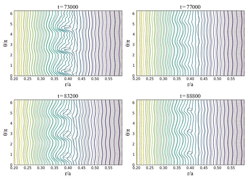
Figure 9. Temporal evolution of the island width and various frequencies for the
oscillated case (ω0 = ωdia0 =12.8 kHz, δBr /B0 = 9.75 × 10⁻⁵ ) in figure 8. Oscillation of
ωdia is observed after mode penetration. Four time points t=73000, t=77000, t=83200
and t=88800 are marked by the red circles.
Figure 10. Contour plot of the plasma pressure p (solid lines) and poloidal flux ψ
(dotted lines), corresponding to the four red time points marked in figure 9.12
0.10
fb = 0.3
0.05 fb = 0.2
0.08
fb = 0.1
0.04
LVODQGZLGWK
LVODQGZLGWK
0.06
0.03
0.04
0.02
η = 1 × 10⁻⁶
0.02 η = 2 × 10⁻⁶ 0.01
η = 3 × 10⁻⁶
0.00 0.00
0 25000 50000 75000 100000 125000 150000 0 25000 50000 75000 100000 125000 150000
WIJ WIJ
D D
0.05 0.05
0.04 0.04
LVODQGZLGWK
LVODQGZLGWK
0.03 0.03
0.02 0.02
χ ∥ = 10, χ ⟂ = 5 × 10⁻⁶ χ ∥ = 10, χ ⟂ = 5 × 10⁻⁶
0.01 χ ∥ = 7, χ ⟂ = 5 × 10⁻⁶ 0.01 χ ∥ = 10, χ ⟂ = 6 × 10⁻⁶
χ ∥ = 5, χ ⟂ = 5 × 10⁻⁶ χ ∥ = 10, χ ⟂ = 7 × 10⁻⁶
0.00 0.00
0 25000 50000 75000 100000 125000 150000 0 25000 50000 75000 100000 125000 150000
WIJ WIJ
D D
Figure 11. Comparison of island width versus time for different (upper left) resistivity
η, (upper right) bootstrap current fraction fb , (lower left) parallel transport coefficient
χk and (lower right) perpendicular transport coefficient χ⊥ .
threshold is almost the same. However, there are two differences observed. First, the
saturated island width is evidently smaller for the case (ωE0 =0, ωdia0 =12.8 kHz) than
that of the case (ωE0 =12.8 kHz, ωdia0 =0), implying that the diamagnetic flow can drive
a stabilizing effect on the magnetic island. Second, an oscillation phenomenon of the
magnetic island is discovered after mode penetration. To further analyze this oscillation
phenomenon, the island width and flow frequency of the oscillated case in figure 8 are
plotted, as shown in figure 9. The periodical oscillation of diamagnetic flow frequency is
observed as well in figure 9 (right). It should be noted that the oscillation of frequency
lags behind the island width a bit, suggesting that the change of island width results
in the change of the diamagnetic flow frequency at first. Since the diamagnetic flow
is proportional to the pressure gradient, it can be straightforwardly inferred that this
phenomenon is related to the change of plasma pressure. To proceed a further step,
the contour plot of the pressure p together with the poloidal magnetic flux ψ is shown
in figure 10, corresponding to the four red time points in figure 9. As the magnetic
island grows larger (t=73000 and t=83200), the pressure gradient ∇k p with respect to
the magnetic field inside the island becomes larger. For a smaller island width (t=77000
and t=88800), on the contrary, the ∇k p is smaller. This modification of pressure gradient
can in return affect the island width by the δ∇k p term in equation (2), leading to the13
above oscillation phenomenon.
In order to further verify our conjecture, the effect of resistivity η is then
investigated. For a larger η, it turns out that the oscillation phenomenon disappears
and the island width recovers as illustrated in figure 11 (upper left). It can be easily
understood through equation (2). Since η is a diffusive term , the effect of δ∇k p term,
stabilizing the island and causing the oscillation, can be diffused to some extent with the
increasing η, in much the same way as viscosity ν in the vorticity equation stabilizing
the oscillation of rotation. In other words, the oscillation phenomenon is a result of
the competition of the two terms δ∇k p and η(j − jb ). For the same reason, a smaller
bootstrap current fraction fb can remove the oscillation by making the η(j − jb ) term
larger, shown in figure 11 (upper right). As the ratio of parallel to perpendicular
transport coefficient χk /χ⊥ is crucial to the process of pressure evolution, the effect of
different χk and χ⊥ values are studied. In figure 11 (lower left and right), the temporal
evolution of the island width is plotted for different χk and χ⊥ . The results are intuitive,
i.e. a smaller χk or larger χ⊥ can eliminate the oscillation. This is because a smaller
χk /χ⊥ can lower the energy transport level along the magnetic field lines, which would
reduce the variation of δ∇k p term when the size of magnetic island changes.
4. Summary and discussion
The initial value code MDC (MHD@Dalian Code) is upgraded with the capability of
two-fluid effects. On the basis of the well-known four-field equations [40], the bootstrap
current, parallel and perpendicular transport effects are additionally included. In this
paper, the numerical simulation on the mode penetration is conducted based on the
two-fluid model. Main points can be summarized as follows.
(i) The threshold of mode penetration at zero rotation is explored. It is found that for
the classical TM (fb = 0), there is not a threshold for mode penetration. At this
circumstance, the behavior of magnetic island is dominated by driven reconnection,
i.e. the saturated island width is positively related to the amplitude of RMP.
For the NTM (fb = 0), on the other hand, a mode penetration like phenomenon
is observed consisting of a driven reconnection regime and a NTM regime. This
phenomenon is different from the so-called mode penetration, but can be mistakenly
defined as mode penetration if not carefully distinguished. It may provide a possible
explanation for the finite mode penetration threshold at zero rotation detected in
experiments.
(ii) The effect of diamagnetic drift flow on the mode penetration is numerically studied.
For a smaller diamagnetic drift flow, numerical results show that its influence is
almost the same as the electric drift flow with comparable frequency. However,
for a larger diamagnetic drift flow, it can drive a stabilizing effect on the magnetic
island through the δ∇k p term in equation (2). Besides, an oscillation phenomenon of
the island width is observed. This oscillation is linked with the change of pressure14
during the variation of island width. It tends to appear in the high Lundquist
number S and high χk /χ⊥ regime, where the parameter of advanced tokamak
exactly lies in.
It should be pointed out that, in our simulation, the resistivity η is set as a constant.
On more realistic regards, η is related to the temperature and can be estimated by the
following equation
πe2 m1/2
η≈ ln Λ, (8)
(4πε0 )2 (KTe )3/2
where ln Λ is a correction factor due to small-angle collisions and is approximate to 16 in
fusion plasmas. In addition, bremsstrahlung radiation of ions and impurities inside the
magnetic island [46] can radiate considerable energy and make significant modification
to the pressure profile, which can directly affect the bootstrap current and increase the
resistivity inside the island. These effects will be included in our future study.
Acknowledgements
We acknowledge the Super Computer Center of Dalian University of Technology for
providing computer resources. This work is supported by National Natural Science
Foundation of China (Grant Nos. 11925501 and 12075048) and Fundamental Research
Funds for the Central Universities (Grant No. DUT21GJ204).
References
[1] Furth H P, Killeen J and Rosenbluth M N 1963 The Physics of Fluids 6 459–484 (Preprint
https://aip.scitation.org/doi/pdf/10.1063/1.1706761) URL https://aip.scitation.
org/doi/abs/10.1063/1.1706761
[2] Rutherford P H 1973 The Physics of Fluids 16 1903–1908 (Preprint https://aip.scitation.
org/doi/pdf/10.1063/1.1694232) URL https://aip.scitation.org/doi/abs/10.1063/1.
1694232
[3] Carrera R, Hazeltine R D and Kotschenreuther M 1986 The Physics of Fluids 29 899–902 (Preprint
https://aip.scitation.org/doi/pdf/10.1063/1.865682) URL https://aip.scitation.
org/doi/abs/10.1063/1.865682
[4] Bardóczi L, Rhodes T L, Bañón Navarro A, Sung C, Carter T A, La Haye R J, McKee
G R, Petty C C, Chrystal C and Jenko F 2017 Physics of Plasmas 24 056106 (Preprint
https://doi.org/10.1063/1.4977533) URL https://doi.org/10.1063/1.4977533
[5] Wang Z X, Wei L and Yu F 2015 Nuclear Fusion 55 043005 URL https://doi.org/10.1088%
2F0029-5515%2F55%2F4%2F043005
[6] Zhang W, Ma Z W, Zhu J and Zhang H W 2019 Plasma Physics and Controlled Fusion 61 075002
URL https://doi.org/10.1088%2F1361-6587%2Fab16ae
[7] La Haye R J 2006 Physics of Plasmas 13 055501 (Preprint https://doi.org/10.1063/1.
2180747) URL https://doi.org/10.1063/1.2180747
[8] Sauter O, Henderson M A, Ramponi G, Zohm H and Zucca C 2010 Plasma Physics and Controlled
Fusion 52 025002 URL https://doi.org/10.1088%2F0741-3335%2F52%2F2%2F025002
[9] Maraschek M 2012 Nuclear Fusion 52 074007 URL https://doi.org/10.1088%2F0029-5515%
2F52%2F7%2F07400715
[10] Hender T, Fitzpatrick R, Morris A, Carolan P, Durst R, Edlington T, Ferreira J, Fielding S,
Haynes P, Hugill J, Jenkins I, Haye R L, Parham B, Robinson D, Todd T, Valovic M and
Vayakis G 1992 Nuclear Fusion 32 2091–2117 URL https://doi.org/10.1088%2F0029-5515%
2F32%2F12%2Fi02
[11] Yu Q, Günter S and Finken K H 2009 Physics of Plasmas 16 042301 (Preprint https://doi.
org/10.1063/1.3100236) URL https://doi.org/10.1063/1.3100236
[12] Buttery R, Benedetti M D, Gates D, Gribov Y, Hender T, Haye R L, Leahy P, Leuer J, Morris
A, Santagiustina A, Scoville J, Tubbing B, Team J, Team C D R and Team D D 1999 Nuclear
Fusion 39 1827–1835 URL https://doi.org/10.1088/0029-5515/39/11y/323
[13] Lanctot M, Olofsson K, Capella M, Humphreys D, Eidietis N, Hanson J, Paz-Soldan C, Strait E
and Walker M 2016 Nuclear Fusion 56 076003 URL https://doi.org/10.1088/0029-5515/
56/7/076003
[14] Logan N, Zhu C, Park J K, Yang S and Hu Q 2021 Nuclear Fusion 61 076010 URL https:
//doi.org/10.1088/1741-4326/abff05
[15] Nave M and Wesson J 1990 Nuclear Fusion 30 2575–2583 URL https://doi.org/10.1088/
0029-5515/30/12/011
[16] Lu S S, Ma Z W, Zhang H W and Liu Y 2020 Plasma Physics and Controlled Fusion 62 125005
URL https://doi.org/10.1088/1361-6587/abbcc4
[17] Wang H, Wang Z, Ding Y and Rao B 2015 Plasma Science and Technology 17 539–544 URL
https://doi.org/10.1088/1009-0630/17/7/03
[18] Wolf R, Biel W, Bock M D, Finken K, Günter S, Hogeweij G, Jachmich S, Jakubowski M,
Jaspers R, Krmer-Flecken A, Koslowski H, Lehnen M, Liang Y, Unterberg B, Varshney S,
von Hellermann M, Yu Q, Zimmermann O, Abdullaev S, Donné A, Samm U, Schweer B,
Tokar M, Westerhof E and the TEXTOR Team 2005 Nuclear Fusion 45 1700–1707 URL
https://doi.org/10.1088/0029-5515/45/12/026
[19] Choi W, La Haye R J, Lanctot M J, Olofsson K E, Strait E J, Sweeney R and Volpe F A 2018
Nuclear Fusion 58 aaa6e3 ISSN 17414326 URL https://doi.org/10.1088/1741-4326/aaa6e3
[20] Tang W, Wang Z X, Wei L, Wang J and Lu S 2020 Nuclear Fusion 60 026015 URL https:
//doi.org/10.1088/1741-4326/ab61d5
[21] Nelson A O, Logan N C, Choi W, Strait E J and Kolemen E 2020 Plasma Physics and Controlled
Fusion 62 094002 URL https://doi.org/10.1088/1361-6587/ab9b3b
[22] Fitzpatrick R 1993 Nuclear Fusion 33 1049–1084 URL https://doi.org/10.1088/0029-5515/
33/7/i08
[23] Yu Q and Günter S 2008 Nuclear Fusion 48 065004 URL https://doi.org/10.1088/0029-5515/
48/6/065004
[24] Cole A J, Hegna C C and Callen J D 2007 Phys. Rev. Lett. 99(6) 065001 URL https:
//link.aps.org/doi/10.1103/PhysRevLett.99.065001
[25] Wang J, Wang Z X and Wei L 2015 Physics of Plasmas 22 092122 (Preprint https://doi.org/
10.1063/1.4931067) URL https://doi.org/10.1063/1.4931067
[26] Beidler M T, Callen J D, Hegna C C and Sovinec C R 2018 Physics of Plasmas 25 082507 (Preprint
https://doi.org/10.1063/1.5046076) URL https://doi.org/10.1063/1.5046076
[27] Zhang H W, Lin X, Ma Z W, Zhang W and Bagwell T E 2021 Plasma Physics and Controlled
Fusion 63 035011 URL https://doi.org/10.1088/1361-6587/abd304
[28] Becoulet M, Orain F, Maget P, Mellet N, Garbet X, Nardon E, Huysmans G, Casper T, Loarte
A, Cahyna P, Smolyakov A, Waelbroeck F, Schaffer M, Evans T E, Liang Y, Schmitz O,
Beurskens M, Rozhansky V and Kaveeva E 2012 Nuclear Fusion 52 054003 URL http:
//doi.org/10.1088/0029-5515/52/5/054003
[29] Yu Q, Günter S and Lackner K 2018 Nuclear Fusion 58 054003 URL https://doi.org/10.1088%
2F1741-4326%2Faab2fb
[30] Fitzpatrick R 2018 Physics of Plasmas 25 082513 (Preprint https://doi.org/10.1063/1.
5043203) URL https://doi.org/10.1063/1.504320316
[31] Fitzpatrick R 2018 Physics of Plasmas 25 112505 (Preprint https://doi.org/10.1063/1.
5053804) URL https://doi.org/10.1063/1.5053804
[32] Yu Q, Günter S and Lackner K 2021 Nuclear Fusion 61 036040 URL https://doi.org/10.1088/
1741-4326/abd197
[33] Hu Q, Logan N, Park J K, Paz-Soldan C, Nazikian R and Yu Q 2020 Nuclear Fusion 60 076006
URL https://doi.org/10.1088/1741-4326/ab8b79
[34] Bock M D, Classen I, Busch C, Jaspers R, Koslowski H and and B U 2008 Nuclear Fusion 48
015007 URL https://doi.org/10.1088/0029-5515/48/1/015007
[35] Wei L, Wang Z X, Wang J and Yang X 2016 Nuclear Fusion 56 106015 URL http://stacks.iop.
org/0029-5515/56/i=10/a=106015?key=crossref.51a4d6ebf40ee4461b4ad0b15ca7f588
[36] Wang J, Wang Z X, Wei L and Liu Y 2017 Nuclear Fusion 57 046007 URL http://stacks.iop.
org/0029-5515/57/i=4/a=046007?key=crossref.6d879fa2ab17585f1e3b54ac2dcce45b
[37] Liu T, Wang Z X, Wang J and Wei L 2018 Nuclear Fusion 58 076026 URL https://doi.org/
10.1088%2F1741-4326%2Faac527
[38] Ye C, Wang Z X, Wei L and Hu Z Q 2019 Nuclear Fusion 59 096044 URL http://iopscience.
iop.org/10.1088/1741-4326/ab3000
[39] Han M, Wang Z X, Dong J and Du H 2017 Nuclear Fusion 57 046019 URL https://doi.org/
10.1088/1741-4326/aa5d02
[40] Hazeltine R D, Kotschenreuther M and Morrison P J 1985 The Physics of Fluids 28 2466–
2477 (Preprint https://aip.scitation.org/doi/pdf/10.1063/1.865255) URL https://
aip.scitation.org/doi/abs/10.1063/1.865255
[41] Bickerton R J, Connor J W and Taylor J B 1971 Nature Physical Science 229 110–112 URL
https://doi.org/10.1038/physci229110a0
[42] Kikuchi Y, De Bock M F M, Finken K H, Jakubowski M, Jaspers R, Koslowski H R, Kraemer-
Flecken A, Lehnen M, Liang Y, Matsunaga G, Reiser D, Wolf R C and Zimmermann O
(TEXTOR-team) 2006 Phys. Rev. Lett. 97(8) 085003 URL https://link.aps.org/doi/10.
1103/PhysRevLett.97.085003
[43] Hu Q, Yu Q, Rao B, Ding Y, Hu X and Zhuang G 2012 Nuclear Fusion 52 083011 URL
http://doi.org/10.1088/0029-5515/52/8/083011
[44] Tang W, Wei L, Wang Z, Wang J, Liu T and Zheng S 2019 Plasma Science and Technology 21
065103 URL https://doi.org/10.1088%2F2058-6272%2Fab0a18
[45] Fitzpatrick R 1998 Physics of Plasmas 5 3325–3341 (Preprint https://doi.org/10.1063/1.
873000) URL https://doi.org/10.1063/1.873000
[46] Gates D A and Delgado-Aparicio L 2012 Phys. Rev. Lett. 108(16) 165004 URL https://link.
aps.org/doi/10.1103/PhysRevLett.108.165004You can also read