Anisotropic viscoacoustic wave modelling in VTI media using frequency-dependent complex velocity

Journal of Geophysics and Engineering
Journal of Geophysics and Engineering (2020) 17, 700–717 doi:10.1093/jge/gxaa023

Anisotropic viscoacoustic wave modelling in VTI
media using frequency-dependent complex velocity
 1,2 1,2,3, 1,2
Yabing Zhang , Yang Liu * and Shigang Xu
1
 State Key Laboratory of Petroleum Resources and Prospecting, China University of Petroleum (Beijing),

 Downloaded from https://academic.oup.com/jge/article/17/4/700/5863467 by guest on 22 December 2020
Beijing, 102249, China
2
 CNPC Key Laboratory of Geophysical Prospecting, China University of Petroleum (Beijing), Beijing,
102249, China
3
 China University of Petroleum (Beijing), Karamay Campus, Karamay, Xinjiang, 834000, China

*Corresponding author: Yang Liu. E-mail: wliuyang@vip.sina.com

Received 17 December 2019, revised 10 March 2020
Accepted for publication 28 April 2020

Abstract
Under the conditions of acoustic approximation and isotropic attenuation, we derive the pseudo-
and pure-viscoacoustic wave equations from the complex constitutive equation and the
decoupled P-wave dispersion relation, respectively. Based on the equations, we investigate the
viscoacoustic wave propagation in vertical transversely isotropic media. The favourable
advantage of these formulas is that the phase dispersion and the amplitude dissipation terms are
inherently separated. As a result, we can conveniently perform the decoupled viscoacoustic
wavefield simulations by choosing different coefficients. In the computational process, a
generalised pseudo-spectral method and a low-rank decomposition scheme are adopted to
calculate the wavenumber-domain and mixed-domain propagators, respectively. Because
low-rank decomposition plays an important role in the simulated procedure, we evaluate the
approximation accuracy for different operators using a linear velocity model. To demonstrate the
effectiveness and the accuracy of our method, several numerical examples are carried out based
on the new pseudo- and pure-viscoacoustic wave equations. Both equations can effectively
describe the viscoacoustic wave propagation characteristics in vertical transversely isotropic
media. Unlike the pseudo-viscoacoustic wave equation, the pure-viscoacoustic wave equation
can produce stable viscoacoustic wavefields without any SV-wave artefacts.
Keywords: complex velocity, pseudo-viscoacoustic, pure-viscoacoustic, generalised
pseudo-spectral method, low-rank decomposition

1. Introduction
The ubiquitous seismic anisotropy is deemed as an important property that has an effect on wave propagation and reverse-
time migration. Generally, there are several numerical algorithms to achieve the wavefield simulation in anisotropic media.
A typical approach is to directly solve the full elastic wave equations and then decouple the wavefield into P- and S-wave
components. However, the wavefield separation in heterogeneous anisotropic media is very complicated and extremely com-
putational inefficient (Yan & Sava 2009; Xu & Zhou 2014; Wang et al. 2016).
 Given this problem, some scholars propose to simulate the P-wave propagation using a pseudo-acoustic (PSA) wave equa-
tion, which is derived from the acoustic approximation (Alkhalifah 1998, 2000; Du et al. 2007; Fowler et al. 2010). Rao &
Wang (2019) explicitly derive the numerical dispersion relation and stability condition for the PSA wave equation. Compared

700 © The Author(s) 2020. Published by Oxford University Press on behalf of the Sinopec Geophysical Research Institute. This is an Open Access article distributed under the terms of
 the Creative Commons Attribution License (http://creativecommons.org/licenses/by/4.0/), which permits unrestricted reuse, distribution, and reproduction in any medium,
 provided the original work is properly cited.

Journal of Geophysics and Engineering (2020) 17, 700–717 Zhang et al.

with the elastic case, this approach can effectively implement P-wave propagation and largely reduce the computational cost.
Unfortunately, setting SV-wave velocity to zero along the axis cannot completely eliminate the SV-wave artefacts in all direc-
tions (Grechka & Tsvankin 2004; Chu et al. 2011; Xu & Liu 2018). On the contrary, the pure-acoustic (PUA) wave equation,
derived from the decoupled P-wave dispersion relation, provides a stable and SV-wave free solution for the acoustic wavefield
simulation in anisotropic media (Chu et al. 2011; Xu & Zhou 2014; Yan & Liu 2016).
 The currently available modelling approaches for anisotropic acoustic wave usually ignore the attenuating effects of the
real Earth materials. However, seismic wave propagation in attenuating media usually suffers from amplitude dissipation and
phase dispersion (Wang & Guo 2004; Wang 2008; Guo et al. 2016; Chen et al. 2019). Without properly considering the
attenuating effects, poor illuminations and incorrect structural positions may occur in migrated image (Sun et al. 2016; Guo
& McMechan 2018; Sun & Zhu 2018).
 So far, there are mainly three kinds of theory to describe the attenuating behaviours in the numerical simulation. The
first method, based on the constant-Q model, gives a convenient description about seismic attenuation (Kjartansson 1979).
Under this theory, the relation between stress and strain is expressed as a convolution operator, which can be computed by

 Downloaded from https://academic.oup.com/jge/article/17/4/700/5863467 by guest on 22 December 2020
fractional time derivatives (Caputo & Mainardi 1971; Podlubny 1999; Carcione et al. 2002; Carcione 2009). It is notable
that solving the fractional time derivative requires storing whole previous wavefields, which is unacceptable for practical cal-
culation. To overcome this limitation, Carcione (2010) adopts fractional Laplacians to replace fractional time derivatives.
Following Carcione’s work, Zhu & Harris (2014) further derive a viscoacoustic wave equation with decoupled phase dis-
persion and amplitude dissipation terms. This novel formulation makes it convenient to compensate for energy loss during
wavefield backward propagation (Zhu 2014; Sun et al. 2015; Sun & Zhu 2018). On the other hand, the fractional Laplacians
associated with phase dispersion and amplitude dissipation are spatially varied. Commonly, they can be calculated by locally
homogeneous approximations (Zhu & Harris 2014), constant-order fractional derivative polynomials (Chen et al. 2016; Li
et al. 2016; Wang et al. 2018) or low-rank decompositions (Chen et al. 2016; Sun et al. 2016).
 The second approach to simulate Q effects is based on the generalised standard linear solid theory. Using a series of stan-
dard linear solid elements can closely approximate the constant-Q model over a specific frequency range (Day & Minster
1984; Carcione et al. 1988; Blanch et al. 1995). However, the related equation does not explicitly contain a quality factor,
instead, it is replaced with a set of optimised relaxation times (Emmerich & Korn 1987; Liao & McMechan 1996; Zhu et al.
2013). Moreover, it will increase the complexity of the viscoacoustic wave equations when multiple elements are adopted
to approximate the constant-Q model in a certain frequency band. Simultaneously, the separation of phase dispersion and
amplitude dissipation in viscoaoustic wave equation becomes much harder (Zhu et al. 2014; Yang & Zhu 2018a).
 The third effective methodology depicts the attenuating property by using a complex velocity (Aki & Richards 2002).
Based on this theory, Yang & Zhu (2018a) derive a novel viscoacoustic wave equation to simulate the wavefield propagation
in the time domain. Analogous to the viscoacoustic wave equation derived by Zhu & Harris (2014), this new expression
also contains a real part and an imaginary part, which correspond to the phase dispersion and the amplitude dissipation,
respectively. However, the equation derived by Zhu & Harris (2014) includes two variable-order fractional Laplacian op-
erators, which are determined by wavenumbers and quality factors. Calculating the fractional operators with a low-rank de-
composition method would consume many computational resources. Based on the approximation of angular frequency, the
wavenumber and the velocity are separated from each other. Thus, the calculation of the new complex-valued time-domain
viscoacoustic wave equation is more flexible and more efficient. Based on the new equation, Yang & Zhu (2018b) further de-
velop a viscoacoustic reverse-time migration approach to correct the phase dispersion and the amplitude dissipation caused
by seismic attenuation, and thus, obtain the subsurface migration profiles with accurate spatial locations as well as amplitudes.
 To simulate the attenuating mechanism in anisotropic media, Bai & Tsvankin (2016) present a 2D time-domain finite-
difference algorithm for viscoelastic wavefield simulation in vertical transversely isotropic (VTI) attenuating media. Zhu
(2017) derives the viscoelastic wave equations based on the fractional time derivatives. By transforming fractional time
derivatives into fractional Laplacians, Zhu & Bai (2019) further implement wavefield simulation in VTI attenuating me-
dia. Moreover, Silva et al. (2019) also develop a system of viscoacoustic wave equations to simulate the viscoacoustic wave
propagation in VTI media. However, all of these approaches use either standard linear solid theory or a fractional Laplacian
method.
 In this paper, we first introduce a complex velocity to describe the attenuating property. Second, we derive the novel
pseudo-viscoacoustic (PSVA) and pure-viscoacoustic (PUVA) wave equations in VTI media from the complex constitutive
equation and decoupled P-wave dispersion relation, respectively. Third, a generalised pseudo-spectral method and a low-rank
decomposition scheme are introduced to solve the wavenumber-domain and mixed-domain operators, respectively. Fourth,
we carry out accuracy analyses in terms of several operators with a linear velocity model based on low-rank approximation.

 701

Journal of Geophysics and Engineering (2020) 17, 700–717 Zhang et al.

Fifth, three numerical examples are adopted to prove the applicability and the validity of our new approach during viscoa-
coustic wavefield simulation. Finally, conclusions are summarised based on analyses and experiments.

2. Theory and method
2.1. Pseudo-viscoacoustic wave equations
Based on acoustic approximation, the stress–strain relationship for VTI elastic media can be symbolically written as
 √
 ⎡ 11 ⎤ ⎡ VP2 (1 + 2 ) VP2 (1 + 2 ) VP2 (1 + 2 )⎤ ⎡e11 ⎤
 ⎢ ⎥ ⎢ √ ⎥⎢ ⎥
 ⎢ 22 ⎥ = ⎢ VP2 (1 + 2 ) VP2 (1 + 2 ) VP2 (1 + 2 )⎥ ⎢e22 ⎥ , (1)
 ⎢ ⎥ ⎢ 2√ √ ⎥ ⎢e ⎥
 ⎣ 33 ⎦ ⎣V (1 + 2 ) V 2 (1 + 2 )
 P P V2 ⎦ ⎣ 33 ⎦ P

 Downloaded from https://academic.oup.com/jge/article/17/4/700/5863467 by guest on 22 December 2020
where is the density, ij and eij are the components of stress and strain tensor, VP is the velocity along symmetry axis and
 and are the Thomsen (1986) anisotropy parameters. To simulate the attenuating property of viscoacoustic wave propa-
gation, a frequency-dependent complex velocity is introduced in the frequency domain (Aki & Richards 2002; Yang & Zhu
2018a):
 [ ]
 1 | | isgn( )
 V(x, ) = V0 (x) 1 + ln | | − , (2)
 Q (x) || 0 || 2Q (x)
where x is the spatial coordinate,
 √ is the angular frequency, 0 denotes the reference angular frequency, V0 is a reference
velocity at 0 and i = −1 is the imaginary unit. The conspicuous advantage of equation (2) is that the phase dispersion
and the amplitude dissipation terms are inherently decoupled. Here, (1 + Q1
 ln | |) is related to the phase dispersion, and
 0
isgn( )
 Q
 associates with amplitude dissipation.
 In an elastic medium, the bulk modulus is defined as

 M0 = V02 . (3)

Combining equations (2) and (3), and neglecting high-order terms with respect to Q, we can formulate the complex bulk
modulus as follow
 [ ]
 2 | | isgn( )
 MC = V0 1 +
 2
 ln | | − . (4)
 Q || 0 || Q
Taking the isotropic quality factor into account, we get the following relation in attenuating media based on equations
(1–4):

 ⎡ 11 ⎤ ⎡D11 D11 D13 ⎤ ⎡e11 ⎤
 ⎢ ⎥ ⎢ ⎥⎢ ⎥
 ⎢ 22 ⎥ = ⎢D11 D11 D13 ⎥ ⎢e22 ⎥ , (5)
 ⎢ ⎥ ⎢D D13 D33 ⎥⎦ ⎢⎣e33 ⎥⎦
 ⎣ 33 ⎦ ⎣ 13
in which
 [ ]
 2 | | isgn( )
 D11 = VP2 1+ ln | | − (1 + 2 ) , (6)
 Q || 0 || Q

 [ ]
 2 | | isgn( ) √
 D13 = VP2 1+ ln | | − (1 + 2 ), (7)
 Q || 0 || Q

 [ ]
 2 | | isgn( )
 D33 = VP2 1 + ln || || − . (8)
 Q | 0 | Q
 702

Journal of Geophysics and Engineering (2020) 17, 700–717 Zhang et al.

 (a) (b)

 0 0
 Phase Angle (degrees)

 0.0199

 Phase Angle (degrees)
 0.04
 45 45
 0.0052 0.02
 90 90
 –0.0095 0
 135 135
 –0.0242 –0.02
 180 180
 4500 –0.0389 4500
 4000 –0.04
 0.3 4000 0.3
 0.15 0.15
 3000 0 3000 0
 Velocity (m s–1) 0.15 Velocity (m s–1)
 2000 –0.3
 Epsilon 0.15 Epsilon
 2000 – 0.3

 Downloaded from https://academic.oup.com/jge/article/17/4/700/5863467 by guest on 22 December 2020
Figure 1. Error variations for phase dispersion (a) and amplitude dissipation (b) with reference velocities, phase angles and anisotropy parameters. Note
that the model is an elliptically anisotropic medium.

Equation (5) has a similar structure to that of PSA wave equation in transversely isotropic (TI) media. After some transfor-
mations, we can obtain the equivalent 2D PSVA wave equations as follows:
 2 H 2 H 2 V
 = D + D , (9)
 t 2 11
 x2 13
 z2

 2 V 2 H 2 V
 = D + D , (10)
 t 2 13
 x2 33
 z2
where H and V are the stresses in the horizontal and vertical directions, respectively. Based on equations (9) and (10), we
can resolve the PSVA wavefield extrapolation in attenuating media. However, the modelling results of PSVA wave still contain
some undesired SV-wave components. In addition, the stability of these two equations is seriously restricted by the condition
of ≥ (Chu et al. 2011; Xu & Liu 2018). When ignoring the phase dispersion and the amplitude dissipation terms of the
complex velocity, equations (9) and (10) then degenerate into the PSA wave equations.

2.2. Pure-viscoacoustic wave equation
Another effective scheme to implement the acoustic wave propagation is solving the decoupled P-wave dispersion relation
(Tsvankin 1996). For the attenuating media, the complex-valued P-wave phase velocity can be briefly written as follows
(Appendix A):
 2
 2 V 2 ( ) = D11 sin2 + D33 cos2 + [(D11 sin2 − D33 cos2 ) + 4D213 sin2 cos2 ]1∕2 , (11)
where is the phase angle. After some simplifications, equation (11) can be reformulated as follows:

 ⎧ √ ⎫
 √
 D ⎪ [ ] √ 4( − )k 2 k2
 ⎪
 (1 + 2 )kx2 + kz2 + (1 + 2 )kx2 + kz2 √1 − [
 33 x z
 2 = ⎨ ] 2 ⎬, (12)
 2 ⎪ (1 + 2 )kx2 + kz2 ⎪
 ⎩ ⎭
where kx = k sin is the wavenumber in the x direction and kz = k cos is the wavenumber in the z direction. When applying
the first-order Taylor series expansion to approximate the square-root in equation (12) and ignoring the influence of on
denominator, we attain the following PUVA wave equation (Chu et al. 2011; Zhan et al. 2012; Yan & Liu 2016)
 [ ][ ]
 2 | | isgn( ) 2( − )kx2 kz2
 = VP 1 +
 2 2
 ln | | − 2 2
 (1 + 2 )kx + kz − . (13)
 Q || 0 || Q kx2 + kz2

 After that, the PUVA wavefield extrapolation in VTI media can be effectively implemented by solving equation (13).

 703

Journal of Geophysics and Engineering (2020) 17, 700–717 Zhang et al.
 Table 1. Some abbreviations of different numerical methods.

 Abbreviation Meaning

 PSA Pseudo-acoustic wave
 PSVA Pseudo-viscoacoustic wave
 PUA Pure-acoustic wave
 PUVA Pure-viscoacoustic wave

2.3. Numerical implementation
 isgn( )
With respect to the amplitude dissipation term Q
 , we adopt the following approximation (Yang & Zhu 2018a)

 isgn( ) i i 
 = ≈ , (14)

 Downloaded from https://academic.oup.com/jge/article/17/4/700/5863467 by guest on 22 December 2020
 Q Q | | Q |k|VP
where k = (kx , kz ) is the wavenumber vector. Equation (14) can be conveniently computed by using a generalised pseudo-
 2
spectral method. With respect to the dispersion term Q ln | |, the wavenumber and the velocity are coupled in the natural
 0
logarithm, which cannot be straightforwardly computed by Fourier transform (FT). Given this issue, a low-rank decompo-
sition method is introduced to approximate this operator. After that, the mixed-domain propagator can be decomposed into
a separable representation (Engquist & Ying 2009; Fomel et al. 2013):

 ∑ ∑
 M N
 W(x, k) ≈ W(x, km )amn W(xn , k), (15)
 m=1 n=1

where W(x, km ) is a submatrix of W(x, k) that is composed of selected columns related to wavenumbers, W(xn , k) is another
submatrix that comprises selected rows associated with spatial positions and amn is the middle matrix coefficients. The low-
rank approximation is highly accurate. Generally, the parameters M = N = 3 can satisfy the requirement of accuracy well.
 2 
To illustrate the mechanism of low-rank decomposition, we take D11 x2H in equation (9) as an example:
 { [ ] [ ]}
 2 H [ ] 2 | | 1 −k 2
 D11 2 = VP2 (1 + 2 ) F −kx2 F( H ) +
 −1
 F −1
 −kx2 ln || || F( H ) + F −1 x
 F( t H ) ,
 x Q | 0 | Q VP |k|
 (16)
where t denotes the first-order time derivative, F and F denote forward and inverse FTs, respectively. Using a low-rank
 −1

decomposition method to approximate −kx2 ln | |, we have
 0

 [ ] {N }
 | | ∑M
 ∑
 F−1 −kx ln || || F( H ) ≈
 2
 W(x, km ) amn F [W(xn , k)F( H )] .
 −1
 (17)
 | 0 | m=1 n=1

 Analogously, the other terms in equations (9), (10) and (13) also can be calculated by using a generalized pseudo-spectral
method and a low-rank decomposition scheme (Appendix B). For each time circulation, solving equations (9) and (10)
requires four forward FTs and (4 + 2N) inverse FTs, and solving equation (13) requires two forward FTs and (6 + 3N)
inverse FTs. Note that N is a parameter of low-rank decomposition.

2.4. Accuracy analyses
(1) Accuracy analyses for the approximation of ≈ |k|VP

 During the numerical implementation, ≈ |k|VP is adopted to solve PSVA and PUVA wave equations. However, the ap-
proximation has some limitations in anisotropic media. Therefore, the accuracy analyses for this approximation are necessary.
 In an anistropic medium, the relationship between angular frequency and wavenumber is written as:

 = |k( )|v( ), (18)

 704

Journal of Geophysics and Engineering (2020) 17, 700–717 Zhang et al.

 (b)
 (a)
 1.5 10– 8
 1.5
 4.4703
 0.0278

 Velocity (m s–1)
 Velocity (m s–1)

 2.0
 2.0 2.6542
 0.0023

 2.5 0.8382
 2.5 –0.0232

 –0.9779
 –0.0486 3.0
 3.0
 0 –2.7940
 0 –0.0741 0.157 0
 0.157 0 0.157
 0.314
 0.314 0.157
 kz (m–1) 0.157
 0.314
 kz (m–1) 0.157 0.157
 0.314
 0 0
 0.157
 kx (m–1)
 0 0 kx (m–1)

 Downloaded from https://academic.oup.com/jge/article/17/4/700/5863467 by guest on 22 December 2020
 (c)
 (d)
 1.5
 1.5 10– 8
 0.0278
 2.7008
 Velocity (m s–1)

 Velocity (m s–1)
 2.0
 0.0023 2.0
 0.3492

 2.5 –0.0232
 2.5 –2.0024

 –0.0486
 3.0 –4.3539
 3.0
 0 –0.0741
 0 –6.7055
 0.157 0
 0.157 0.157 0
 0.314
 0.314 0.157
 kz (m ) 0.157
 –1 0.314
 0 0
 0.157
 kx (m–1) kz (m–1) 0.157 0.157
 0.314
 0 0 kx (m–1)

 (e) (f)

 1.5 1.5 10– 8

 0.0139 1.6764
 Velocity (m s–1)

 Velocity (m s–1)

 2.0 2.0
 0.0053 0.9313

 2.5 –0.0033 2.5 0.1863

 –0.0118 –0.5588
 3.0 3.0
 0 –0.0204 0 –1.3039
 0.157 0 0.157 0
 0.314 0.157 0.314 0.157
 kz (m–1) 0.157 0.314 kz (m–1) 0.157 0.157
 0.314
 0 0
 0.157
 kx (m–1) 0 0 kx (m–1)

Figure 2. Low-rank approximations (a, c and e) and their corresponding errors (b, d and f) for different mixed-domain operators: (a) and (b) are
 kx2 kz2
computed by kx2 ln | |; (c) and (d) are computed by kz2 ln | | and (e) and (f) are computed by kx2 +kz2
 ln | |. Note that the accurate values of these
 0 0 0
operators are not displayed here.

where v( ) is the phase velocity. Under the acoustic assumption, the phase velocity in VTI media can be expressed as
(Thomsen 1986):

 v2 ( ) ≈ VP2 (1 + sin2 + E( )), (19)

and
 [√ ]
 1
 E( )= 1+(8 − 4 )sin cos + 4 (1 + )sin − 1 .
 2 2 4
 (20)
 2

 705

Journal of Geophysics and Engineering (2020) 17, 700–717 Zhang et al.
 Colorbar

 – 0.2 – 0.1 0.0 0.1 0.2

 (a) Distance (m) (b) Distance (m)
 0 1000 2000 3000 0 1000 2000 3000
 0 0
 PSA PSVA
 Reference

 1000 1000

 Depth (m)
 Depth (m)

 2000 2000

 Downloaded from https://academic.oup.com/jge/article/17/4/700/5863467 by guest on 22 December 2020
 3000 3000

 (c) Distance (m) (d) Distance (m)
 0 1000 2000 3000 0 1000 2000 3000
 0 0
 PSVA PSVA
 Low-rank Difference

 1000 1000
 Depth (m)
 Depth (m)

 2000 2000

 3000 3000
 Distance (m) Distance (m)
 (e) (f)
 0 1000 2000 3000 0 1000 2000 3000
 0 0
 PUA PUVA
 Reference

 1000 1000
 Depth (m)
 Depth (m)

 2000 2000

 3000 3000

 (g) Distance (m) (h) Distance (m)
 0 1000 2000 3000 0 1000 2000 3000
 0 0
 PUVA PUVA
 Low-rank Difference

 1000 1000
 Depth (m)

 Depth (m)

 2000 2000

 3000 3000

Figure 3. Wavefield snapshots computed by PSA (a), PSVA (b and c), PUA (e) and PUVA (f and g) wave equations using the generalised pseudo-
spectral method (a, b, e and f) and the low-rank decomposition scheme (c and g). (d) is the wavefield difference between (b) and (c) and (h) is the
wavefield difference between (f) and (g). Note that all the wavefield snapshots are plotted using the same colorbar.

 706

Journal of Geophysics and Engineering (2020) 17, 700–717 Zhang et al.

 Colorbar

 – 0.2 – 0.1 0.0 0.1 0.2

 (a) Distance (m) (b) Distance (m)
 0 1000 2000 3000 0 1000 2000 3000
 0 0
 Acoustic Dissipation Acoustic Dissipation
 PSVA PUVA

 1000 1000

 Depth (m)
 Depth (m)

 Downloaded from https://academic.oup.com/jge/article/17/4/700/5863467 by guest on 22 December 2020
 2000 2000

 Dispersion Viscoacoustic Dispersion Viscoacoustic
 3000 3000

 (c) Distance (m) (d) Distance (m)
 0 1000 2000 3000 0 1000 2000 3000
 0 0
 Q = 500 Q = 50 Q = 500 Q = 50
 PSVA PUVA

 1000 1000
 Depth (m)
 Depth (m)

 2000 2000

 Q = 100 Q = 20 Q = 100 Q = 20
 3000 3000

Figure 4. Wavefield snapshots of PSVA and PUVA at 0.7 s in a homogeneous medium. (a) and (b) are obtained by using the anisotropic acoustic,
dispersion-effect, dissipation-effect and viscoacoustic wave equations, respectively, and (c) and (d) are obtained by using the viscoacoustic wave equation
with different Q values. Note that all the wavefield snapshots are plotted using the same colorbar.

 ln | |) is related to the phase dispersion, and
 2 isgn( )
 In the complex stiffness coefficients D11 , D13 and D33 , (1 + Q Q
 as-
 0
sociates with the amplitude dissipation. For the phase dispersion term, we have
 ( ) ( ) ( )
 2 | | 2 | |k| v( ) | 2 | |k| VP |
 1+ ln || || = 1+ ln | | ≈ 1+ ln | | . (21)
 Q | 0 | Q || 0 || Q || 0 ||

 Using reference velocity VP to replace phase velocity v( ) in anisotropic media would produce some errors, which can be
defined as follows:

 2 ( | )
 error = ln |v( )|| − ln ||VP || . (22)
 Q

 Based on equation (22), we calculate the errors with different reference velocities, phase angles and anisotropy parameters,
shown in figure 1a (for convenience, the medium is elliptically anisotropic). It can be seen that the approximation error is very
small.

 707

Journal of Geophysics and Engineering (2020) 17, 700–717 Zhang et al.

 (b)
 (a)
 Acoustic Acoustic
 0.8 Dispersion 0.8 Dispersion
 Dissipation Dissipation
 0.4 Viscoacoustic 0.4 Viscoacoustic
 Amplitude

 Amplitude
 0.0 0.0

 –0.4 –0.4

 –0.8 –0.8
 PSVA PUVA

 400 450 500 550 400 450 500 550
 Time (ms) Time (ms)

 Downloaded from https://academic.oup.com/jge/article/17/4/700/5863467 by guest on 22 December 2020
 (c) (d)
 Q = 500 Q = 500
 0.8 Q = 100 0.8 Q = 100
 Q = 50 Q = 50
 0.4 Q = 20 0.4 Q = 20

 Amplitude
 Amplitude

 0.0 0.0

 –0.4 –0.4

 –0.8 –0.8
 PSVA PUVA

 400 450 500 550 400 450 500 550
 Time (ms) Time (ms)

Figure 5. Extracted single traces of PSVA and PUVA at the distance of 750 m in a homogeneous medium. (a) and (b) are calculated by using the
anisotropic acoustic, dispersion-effect, dissipation-effect and viscoacoustic wave equations, respectively, and (c) and (d) are calculated by using the vis-
coacoustic wave equation with different Q values.

 m s–1

 m s–1

Figure 6. Two-layered model.

 Without considering the dispersion effect of complex velocity, we have
 [ ] [ ]
 isgn( ) i 
 1− ≈ 1− . (23)
 Q Q |k| VP
 After importing the approximation ≈ |k|VP , the error of equation (23) can be defined as:
 ( )
 i i i v( )
 error = − = 1− . (24)
 Q |k| v( ) Q |k| VP Q VP

 708

Journal of Geophysics and Engineering (2020) 17, 700–717 Zhang et al.
 Colorbar

 –0.2 –0.1 0.0 0.1 0.2

 (a) Distance (m) (b) Distance (m)
 0 1000 2000 3000 0 1000 2000 3000
 0 0
 PSA PSVA

 1000 1000

 Depth (m)
 Depth (m)

 2000 2000

 Downloaded from https://academic.oup.com/jge/article/17/4/700/5863467 by guest on 22 December 2020
 3000 3000

 (c) Distance (m) (d) Distance (m)
 0 1000 2000 3000 0 1000 2000 3000
 0 0
 PUA PUVA

 1000 1000
 Depth (m)
 Depth (m)

 2000 2000

 3000 3000

Figure 7. Wavefield snapshots at 0.6 s computed by using (a) PSA, (b) PSVA, (c) PUA and (d) PUVA wave equations in a two-layered model. Note that
all the wavefield snapshots are plotted in the same colorbar.

 Ignoring the effect of imaginary unit, the error becomes Q1 (1 − v( )
 VP
 ). Figure 1b displays the corresponding error variations
with reference velocities, phase angles and anisotropy parameters in an elliptically anisotropic medium. Compared with the
value of equation (23), the error is negligible.
 Based on these analyses, we can see that the approximation of ≈ |k|VP is limited in anisotropic media, but the error is
relatively small and thus acceptable under the assumption of weak anisotropy and attenuation.

(2) Accuracy analyses for low-rank decomposition

 To reduce the numerical error caused by computational algorithms, we jointly adopt the pseudo-spectral method and the
low-rank decomposition scheme to solve equations (9), (10) and (13), respectively. For the sake of evaluating the accuracy
of low-rank approximation, we design a simple model with linear velocity, which varies from 1500 to 3000 m·s−1 . Moreover,
the wavenumbers of kx and kz are between 0 and 0.314 m−1 , and the reference frequency is set to 0 = 1000 rad s−1 . Figure 2
 k2 k2
shows the approximations of kx2 ln | |, kz2 ln | | and k2x+kz 2 ln | |, and their corresponding errors using low-rank decom-
 0 0 x z 0
position with M = N = 2. For simplicity, the exact values are not displayed here. From figure 2, we can see that the values of
these three operators are between −0.074 and 0.0278, while their errors are as small as 10−8 . It illustrates that the low-rank
decomposition has very high accuracy.

3. Numerical examples
In this section, three numerical examples are carried out using our proposed PSVA and PUVA wave equations. In each ex-
ample, we set 0 = 1000 rad·s−1 . A Ricker signal with main frequency of 20 Hz is used to produce waves. The parameters
 709

Journal of Geophysics and Engineering (2020) 17, 700–717 Zhang et al.

 Downloaded from https://academic.oup.com/jge/article/17/4/700/5863467 by guest on 22 December 2020

Figure 8. Seismic records computed by using the (a) PSA, (b) PSVA, (c) PUA and (d) PUVA wave equations in a two-layered model. (e) and (f) are
the extracted traces at the distance of 1000 m as indicated by the black dotted lines in (a–d). (g) and (h) are the extracted traces at the time of 500 ms as
indicated by the white dotted lines in (a–d), respectively.

 710

Journal of Geophysics and Engineering (2020) 17, 700–717 Zhang et al.

 Downloaded from https://academic.oup.com/jge/article/17/4/700/5863467 by guest on 22 December 2020
Figure 9. Parameters for the heterogeneous model: (a) v, (b) , (c) and (d) Q.

M = N = 3 are adopted in the low-rank approximation. To eliminate the artefact boundary reflections, a modified hybrid
absorbing boundary condition is applied during the wavefield simulation (Liu & Sen 2010, 2018). For convenience, we first
give some abbreviations of different numerical methods in Table 1.

3.1. A homogeneous model
Our first example is for a 2D homogeneous model with grids of 301 × 301. The grid intervals in the x- and z-directions are
10 m. The velocity along the symmetry axis is 1500 m s−1 . The Thomsen anisotropy parameters are = 0.20 and = 0.15,
respectively. The quality factor is Q = 20. The record length and the time step are 1.2 and 0.001 s, respectively. The source
wavelet is placed at the centre of the model. The reference solution in the homogeneous model is directly computed by us-
ing the generalised pseudo-spectral method. Figure 3 shows several wavefield snapshots and their differences compared with
the reference solutions. Unlike the acoustic modelling wavefields (figure 3a and e), the viscoacoustic modelling wavefields
(figure 3b, c, f and g) have a large amount of energy loss. Besides, the wavefields computed by PSA (figure 3a) and PSVA
(figure 3b and c) wave equations contain some strong SV-wave artefacts around the source, while they are effectively elimi-
nated in the wavefields of PUA (figure 3e) and PUVA (figure 3f and g). In addition, the differences (figure 3d and h) between
the reference solutions (figure 3b and f) and our new modelling results (figure 3c and g) are very small, which illustrates that
our proposed algorithm is highly accurate.
 Because the phase dispersion and the amplitude dissipation are naturally decoupled in the complex velocity, we can conve-
niently implement different viscoacoustic behaviours by choosing different coefficients in equations (9), (10) and (13). For
example, figure 4a and b show four wavefields at 0.7 s, calculated by the anisotropic acoustic, dispersion-effect, dissipation-
effect and viscoacoustic wave equations, respectively. Compared with the acoustic wavefield, the dispersion-effect wavefield
has little amplitude variation, but presents a delayed phase. In contrast, the dissipation-effect wavefield only occurs amplitude

 711

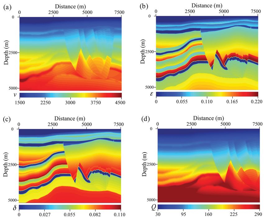
Journal of Geophysics and Engineering (2020) 17, 700–717 Zhang et al.

 Colorbar

 –0.2 – 0.1 0.0 0.1 0.2

 (a) Distance (m) (b) Distance (m)
 0 2500 5000 7500 0 2500 5000 7500
 0 0
 PSA PSVA
 Depth (m)

 Depth (m)
 2500 2500

 Downloaded from https://academic.oup.com/jge/article/17/4/700/5863467 by guest on 22 December 2020
 5000 5000

 (c) Distance (m) (d) Distance (m)
 0 2500 5000 7500 0 2500 5000 7500
 0 0
 PUA PUVA

 Depth (m)
 Depth (m)

 2500 2500

 5000 5000

Figure 10. Wavefield snapshots at 0.9 s obtained by using the (a) PSA, (b) PSVA, (c) PUA and (d) PUVA wave equations in the heterogeneous model.

dissipation without phase dispersion. When the dispersion and dissipation effects are considered, the viscoacoustic wavefield
exhibits amplitude dissipation and phase dispersion. To compare the attenuating effects caused by different quality factors,
we adopt the parameter of Q = 500, 100, 50 and 20 to perform the viscoacoustic wavefield modelling. The corresponding
wavefields are shown in figure 4c and d, which indicate that the effects of amplitude dissipation and phase dispersion in-
crease with the decreasing Q. Some comparisons among different traces at the distance of 750 m (figure 5a–d) also give such
conclusions.

3.2. A two-layered model
The second example is a two-layered model shown in figure 6. The computational area is divided into 301 × 301 grids with a
grid spacing of 10 m. The simulated length is 1.2 s with the time step 0.001 s. The interface is located at the depth of 1600 m.
 Figure 7 displays several snapshots at 0.6 s calculated by using the PSA, PSVA, PUA and PUVA wave equations, respec-
tively. Meanwhile, figure 8 plots the corresponding seismic records and extracted traces at the distance of 1000 m or at the
time of 500 ms, respectively. Compared with acoustic modelling wavefields (figure 7a and c) and records (figure 8a and c),
viscoacoustic simulated wavefields (figure 7b and d) and records (figure 8b and d) present obvious amplitude dissipation.
Besides, seismograms from PSA and PSVA wave equations contain a large amount of SV-wave noise, while those from PUA
and PUVA wave equations are completely free of SV-wave noise.

3.3. A heterogeneous model
To verify the accuracy and the robustness of our new schemes, a part of BP 2007 tilted TI (TTI) model with a constant dip
angle = 0◦ is used to perform the viscoacoustic wavefield simulation. The model is discretised by 501 × 361 with a grid
spacing of 15 m. The record length is 1.5 s. The time step of 0.001 s is applied in the wave propagation. Figure 9 displays

 712

Journal of Geophysics and Engineering (2020) 17, 700–717 Zhang et al.
 Colorbar

 –0.2 –0.1 0.0 0.1 0.2

 (a) Distance (m) (b) Distance (m)
 0 2500 5000 7500 0 2500 5000 7500
 0 0
 PSA PSVA

 Time (ms) 500 500

 Time (ms)
 1000 1000

 Downloaded from https://academic.oup.com/jge/article/17/4/700/5863467 by guest on 22 December 2020
 1500 1500

 (c) Distance (m) (d) Distance (m)
 0 2500 5000 7500 0 2500 5000 7500
 0 0
 PUA PUVA

 500 500
 Time (ms)

 Time (ms)

 1000 1000

 1500 1500

 (e) (f)
 0.6 0.6
 PSA PUA
 PSVA PUVA
 0.4 0.4
 Amplitude
 Amplitude

 0.2 0.2

 0.0 0.0

 –0.2 –0.2

 –0.4 –0.4
 600 800 1000 1200 600 800 1000 1200
 (g) Time (ms) (h) Time (ms)
 0.02 0.02
 PSA PUA
 PSVA PUVA
 0.01 0.01
 Amplitude

 Amplitude

 0.00 0.00

 –0.01 –0.01

 –0.02 –0.02
 900 1000 1100 1200 900 1000 1100 1200
 Time (ms) Time (ms)

Figure 11. Seismic records computed by using the (a) PSA, (b) PSVA, (c) PUA and (d) PUVA wave equations in the heterogeneous model. (e) and (f)
are the extracted traces at the distance of 6000 m as indicated by the black dotted lines in (a–d), respectively. (g) and (h) are the magnification of (e) and
(f).

 713

Journal of Geophysics and Engineering (2020) 17, 700–717 Zhang et al.

some model parameters, including the velocity v along the symmetry axis, the quality factor Q = 14 × (v∕1000)2.2 , and the
Thomsen anisotropy parameters and , respectively. The source signal, represented by a Ricker wavelet, located at (3750,
2175 m), is used to generate the waves.
 Figures 10 and 11 show several snapshots and seismograms for the modified BP 2007 TTI model computed by using the
PSA, PSVA, PUA and PUVA wave equations, respectively. Compared with the acoustic modelling wavefield, the viscoacoustic
modelling wavefield contains some amplitude dissipation effects along the wavefront. This phenomenon can be obviously
observed from the extracted traces at the distance of 6000 m (figure 11e–h). In addition, we also compare the computational
efficiency between PSVA and PUVA wave equations in a personal computer (Intel Core i7-8850H 2.60 GHz). The elapsed
times of PSVA and PUVA wave equations are 511.66 and 713.11 s, respectively.

4. Conclusions
We have derived the new PSVA and PUVA wave equations with isotropic quality factor from the complex constitutive wave

 Downloaded from https://academic.oup.com/jge/article/17/4/700/5863467 by guest on 22 December 2020
equation and the decoupled P-wave dispersion relation. Since phase dispersion and amplitude dissipation terms are inherently
separated in these formulas, we can conveniently realise the decoupled viscoacoustic wavefield extrapolation. During the
numerical implementation, the generalised pseudo-spectral method and the low-rank decomposition scheme were adopted
to solve the wavenumber-domain and mixed-domain propagators, respectively. Meanwhile, we also examined the accuracy of
low-rank approximations for different propagators. Several numerical experiments were performed to prove the validity and
the robustness of our approach. Moreover, we compared the modelling results between PSVA and PUVA wave equations.
Unlike the PSVA wave equation, our PUVA wave equation could obtain stable viscoacoustic wavefield without any SV-wave
artefacts.

Acknowledgements
This work is supported by the National Natural Science Foundation of China (grant nos. 41874144 and 41474110) and the Research
Foundation of China University of Petroleum-Beijing at Karamay (grant no. RCYJ2018A-01–001). Y. Zhang is financially supported by
the China Scholarship Council.
Conflict of interest statement. The authors declare that they have no conflict of interest.

Appendix A. Decoupled P-wave dispersion relation
In attenuating media, the Christoffel equation is generally written as follows:

 ̃ − Ṽ 2 I)U
 (G ̃ = 0, (A1)

where G ̃ is the complex Christoffel matrix that depends on the complex stiffness and the phase direction, Ṽ = ∕k̃ is the
complex velocity, k̃ = k − i is the complex wavenumber, is the attenuation coefficient and Ũ is the displacement vector of
the viscoacoustic plane wave.
 Setting the characteristic determinant of equation (A1) to zero yields the following dispersion relation:

 ̃ − Ṽ 2 I) = 0.
 det(G (A2)

Under the acoustic assumption, the decoupled P-wave velocity in 2D attenuating media is obtained by solving equation (A2):
 [( )2 ]1∕2
 2 V 2 ( ) = D11 sin2 + D33 cos2 + D11 sin2 − D33 cos2 + 4D213 sin2 cos2 . (A3)

Appendix B. Specific implementations for PSVA and PUVA wave equations
Under the acoustic assumption, we derive the PSVA and PUVA wave equations, respectively. In the implementation, a gen-
eralised pseudo-spectral method and a low-rank decomposition scheme are adopted to solve the wavenumber-domain and

 714

Journal of Geophysics and Engineering (2020) 17, 700–717 Zhang et al.

mixed-domain propagators. As for equations (9) and (10), each term can be solved by the following equations:
 { [ ]}
 2 H −1 [ ] 2 −1 | |
 | |
 D11 2 = VP (1 + 2 ) F −kx F( H ) +
 2 2
 F 2
 −kx ln | | F( H )
 x [ 2 Q
 ] | 0 | (B1)
 1 −1 −kx
 − VP (1 + 2 ) Q V F
 2
 |k|
 F( t H ) ,
 P

 √ { [ ]}
 2 V −1 [ ] 2 −1 | |
 | |
 D13 2 = VP 1 + 2 F −kz F( V ) +
 2 2
 F 2
 −kz ln | | F( V )
 z [ −k2 Q
 ] | 0 | (B2)
 √ 1
 − VP 1 + 2 Q V F
 2 −1 z
 |k|
 F( t V ) ,
 P

 √ { [ ]}

 Downloaded from https://academic.oup.com/jge/article/17/4/700/5863467 by guest on 22 December 2020
 2 H −1 [ ] 2 −1 | |
 | |
 D13 2 = VP 1 + 2 F −kx F( H ) +
 2 2
 F 2
 −kx ln | | F( H )
 x [ 2 Q
 ] | 0 | (B3)
 √ 1 −1 −kx
 − VP 1 + 2 Q V F
 2
 |k|
 F( t H ) ,
 P

 { [ ]}
 2 V −1 [ ] 2 −1 | |
 | |
 D33 2 = VP F −kz F( V ) +
 2 2
 F 2
 −kz ln | | F( V )
 z [ −k2 Q
 ] | 0 | (B4)
 2 1
 − VP Q V F −1 z
 |k|
 F( t V ) .
 P

In equations (B1)–(B4), F−1 [−kx2 ln | |F( H )] and F−1 [−kz2 ln | |F( V )] are calculated by using the low-rank decom-
 0 0

positions, and the other terms are computed with a pseudo-spectral method. Therefore, solving PSVA wave equation would
spend twice the low-rank decomposition and four times the pseudo-spectral method.
 To solve equation (13), we have
 { [ ]}
 −1 [ ] −1 [ ]
 2P −kx2 kz2
 = VP (1 + 2 )F −kx F(P) + F −kz F(P) − 2( − )F
 2 2 2 −1
 F(P)
 t 2 |k|2

 ⎧ [ ] [ ]⎫
 −1 | | −1 | |
 2VP2
 ⎪(1 + 2 )F −k 2
 ln | | F(P) + F −k 2
 ln | | F(P) ⎪
 x | 0 | [ z
 ] | 0 |
 +
 Q ⎪⎨ 2 k2
 | | ⎬
 −2( − )F−1 |k|x 2 z ln | | F(P)
 −k
 ⎪ (B5)
 ⎩ | 0 | ⎭
 [ 2 ] [ 2 ]
 ⎧ −1 −kx −1 −kz ⎫
 VP ⎪(1 + 2 ) F |k|
 F( t P) + F |k|
 F( t P) ⎪
 + ⎨ [ −k2 k2 ] ⎬,
 Q ⎪ −2 ( − ) F−1 |k|x 3 z F( t P) ⎪
 ⎩ ⎭
 −k2 k2
where P is the pressure. Similarly, F−1 [−kx2 ln | |F(P)], F−1 [−kz2 ln | |F(P)] and F−1 [ |k|x 2 z ln | |F(P)] are calculated
 0 0 0
by using the low-rank decompositions and the other terms are computed with pseudo-spectral method. So, solving PUVA
wave equation would spend three times the low-rank decomposition and six times the pseudo-spectral method. Based on
these analyses, we can see that the computational cost of PUVA is a little larger than that of the PSVA wave equation.

Appendix C. Theoretical quality factor investigation
For a P-wave, the Christoffel equation can be written as:
 ( )( ) ( )2
 D11 k̃ 2 sin2 − 2 D33 k̃ 2 cos2 − 2 − D13 k̃ 2 sin cos = 0. (C1)

 715

Journal of Geophysics and Engineering (2020) 17, 700–717 Zhang et al.

 Based on the complex stiffness coefficients and the definition of quality factor, we get
 ( )
 | Re (D ) | || 1 + 2 ln || || || ( )
 | ij | | Q | 0 | | 2 || ||
 | |
 Qij = | ( ) | ≈ | ( ) | ≈ Q + ln | | . (C2)
 | Im Dij | || sgn( ) |
 | | 0 |
 | | | − Q |

 For weak attenuation, 2 ln | | ≪ Q and | Im(Dij ) | ≈ Q . Then, equation (C1) can be rewritten as follows (Zhu & Tsvankin
 Re(D )
 0 ij
2006):
 ( )( ) [ ]2
 c11 sin2 1 − 2 + ic11 sin2 2 c33 cos2 1 − 2 + ic33 cos2 2 − c13 sin cos ( 1 + i 2 ) = 0, (C3)
where c11 , c13 and c33 are the corresponding real parts of complex stiffness coefficients D11 , D13 and D33 . Solving equation
(C3) yields

 Downloaded from https://academic.oup.com/jge/article/17/4/700/5863467 by guest on 22 December 2020
 2k 
 1 = k2 − 2 + , (C4)
 Q
 1 [ 2 ]
 2 = k − 2 − 2k . (C5)
 Q
 The only physically meaningful solution of the imaginary part of equation (C3) is 2 = 0, which yields the isotropic ex-
pression for attenuation coefficient as follows:
 (√ )
 =k 1 + Q2 − Q . (C6)

 The normalised attenuation coefficient that defines the rate of amplitude decay per wavelength can be expressed as:
 (√ )
 
 ≡ = 1 + Q2 − Q . (C7)
 k
 Based on equation (C7), we can see that the normalised attenuation coefficient for P-wave in velocity anisotropic media
with isotropic Q is independent of the phase angle. When attenuation is weak (1∕Q ≪ 1), equation (C7) becomes
 1
 ≈ . (C8)
 2Q
Therefore, we deem that the theoretical quality factor is in accordance with isotropic attenuation.

References Chen, H., Zhou, H., Li, Q. & Wang, Y., 2016. Two efficient mod-
 eling schemes for fractional Laplacian viscoacoustic wave equation,
Aki, K. & Richards, P.G., 2002. Quantitative Seismology, 2nd edn, University Geophysics, 81, T233–T249.
 Science Books, Sausalito, CA. Chen, Y., Guo, B. & Schuster, G.T., 2019. Migration of viscoacoustic data
Alkhalifah, T., 1998. Acoustic approximations for processing in trans- using acoustic reverse time migration with hybrid deblurring filters,
 versely isotropic media, Geophysics, 63, 623–631. Geophysics, 84, S127–S136.
Alkhalifah, T., 2000. An acoustic wave equation for anisotropic media, Chu, C., Macy, B.K. & Anno, P.D., 2011. Approximation of pure acoustic
 Geophysics, 65, 1239–1250. seismic wave propagation in TTI media, Geophysics, 76, WB97–WB107.
Bai, T. & Tsvankin, I., 2016. Time-domain finite-difference modeling for Day, S.M. & Minster, J.B., 1984. Numerical simulation of attenuated wave-
 attenuating anisotropic media, Geophysics, 81, C69–C77. field using a Padé approximant method, Geophysical Journal of the Royal
Blanch, J.O., Robertsson, J.O.A. & Symes, W.W., 1995. Modeling of a con- Astronomical Society, 78, 105–118.
 stant Q: methodology and algorithm for an efficient and optimally inex- Du, X., Bancroft, J.C. & Lines, L.R., 2007. Anisotropic reverse-time migra-
 pensive viscoelastic technique, Geophysics, 60, 176–184. tion for tilted TI media, Geophysical Prospecting, 55, 853–869.
Caputo, M. & Mainardi, F., 1971. A new dissipation model based on mem- Emmerich, H. & Korn, M., 1987. Incorporation of attenuation into
 ory mechanism, Pure and Applied Geophysics, 91, 134–147. time-domain computations of seismic wavefields, Geophysics, 52,
Carcione, J.M., 2009. Theory and modeling of constant-Q P- and S-waves 1252–1264.
 using fractional time derivatives, Geophysics, 74, T1–T11. Engquist, B. & Ying, L., 2009. A fast directional algorithm for high fre-
Carcione, J.M., 2010. A generalization of the Fourier pseudospectral quency acoustic scattering in two dimensions, Communications in Math-
 method, Geophysics, 75, A53–A56. ematical Sciences, 7, 327–345.
Carcione, J.M., Cavallini, F., Mainardi, F. & Hanyga, A., 2002. Time- Fomel, S., Ying, L. & Song, X., 2013. Seismic wave extrapolation using
 domain modeling of constant-Q seismic waves using fractional deriva- lowrank symbol approximation, Geophysical Prospecting, 61, 526–536.
 tives, Pure and Applied Geophysics, 159, 1719–1736. Fowler, P.J., Du, X. & Fletcher, R.P., 2010. Coupled equations for re-
Carcione, J.M., Kosloff, D. & Kosloff, R., 1988. Wave propagation simula- verse time migration in transversely isotropic media, Geophysics, 75,
 tion in a linear viscoacoustic medium, Geophysical Journal International, S11–S22.
 93, 393–401.

 716

Journal of Geophysics and Engineering (2020) 17, 700–717 Zhang et al.

Grechka, V. & Tsvankin, I., 2004. Characterization of dipping frac- Wang, N., Zhou, H., Chen, H., Xia, M., Wang, S., Fang, J. & Sun, P., 2018.
 tures in transversely isotropic background, Geophysical Prospecting, 52, A constant fractional-order viscoelastic wave equation and its numerical
 1–10. simulation scheme, Geophysics, 83, T39–T48.
Guo, P. & McMechan, G.A., 2018. Compensating Q effects in viscoelastic Wang, Y., 2008. Seismic Inverse Q Filtering, Blackwell Publishing, Oxford.
 media by adjoint-based least-squares reverse time migration, Geophysics, Wang, Y. & Guo, J., 2004. Modified Kolsky model for seismic attenuation
 83, S151–S172. and dispersion, Journal of Geophysics and Engineering, 1, 187–196.
Guo, P., McMechan, G.A. & Guan, H., 2016. Comparison of two vis- Xu, S. & Liu, Y., 2018. Effective modeling and reverse-time migration for
 coacoustic propagators for Q-compensated reverse time migration, novel pure acoustic wave in arbitrary orthorhombic anisotropic media,
 Geophysics, 81, S281–S297. Journal of Applied Geophysics, 150, 126–143.
Kjartansson, E., 1979. Constant Q-wave propagation and attenuation, Xu, S. & Zhou, H., 2014. Accurate simulations of pure quasi-P-waves in
 Journal of Geophysical Research, 84, 4737–4748. complex anisotropic media, Geophysics, 79, T341–T348.
Li, Q., Zhou, H., Zhang, Q., Chen, H. & Sheng, S., 2016. Efficient reverse Yan, J. & Liu, H., 2016. Modeling of pure acoustic wave in tilted trans-
 time migration based on fractional Laplacian viscoacoustic wave equa- versely isotropic media using optimized pseudo-differential operators,
 tion, Geophysical Journal International, 204, 488–504. Geophysics, 81, T91–T106.
Liao, Q. & McMechan, G.A., 1996. Multifrequency viscoacoustic model- Yan, J. & Sava, P., 2009. Elastic wave-mode separation for VTI media,

 Downloaded from https://academic.oup.com/jge/article/17/4/700/5863467 by guest on 22 December 2020
 ing and inversion, Geophysics, 61, 1371–1378. Geophysics, 74, WB19–WB32.
Liu, Y. & Sen, M.K., 2010. A hybrid scheme for absorbing edge re- Yang, J. & Zhu, H., 2018a. A time-domain complex-valued wave equa-
 flections in numerical modeling of wave propagation, Geophysics, 75, tion for modelling visco-acoustic wave propagation, Geophysical Journal
 A1–A6. International, 215, 1064–1079.
Liu, Y. & Sen, M.K., 2018. An improved hybrid absorbing boundary condi- Yang, J. & Zhu, H., 2018b. Viscoacoustic reverse time migration using
 tion for wave equation modeling, Journal of Geophysics and Engineering, a time-domain complex-valued wave equation, Geophysics, 83, S505–
 15, 2602–2613. S519.
Podlubny, I., 1999. Fractional Differential Equations: An Introduction to Frac- Zhan, G., Pestana, R.C. & Stoffa, P.L., 2012. Decoupled equations for re-
 tional Derivatives, Fractional Differential Equations, to Methods of their So- verse time migration in tilted transversely isotropic media, Geophysics,
 lution and Some of their Applications, Academic Press, San Diego, CA. 77, T37–T45.
Rao, Y. & Wang, Y., 2019. Dispersion and stability condition of seismic Zhu, T., 2014. Time-reverse modelling of acoustic wave propagation in at-
 wave simulation in TTI media, Pure and Applied Geophysics, 176, 1549– tenuating media, Geophysical Journal International, 197, 483–494.
 1559. Zhu, T., 2017. Numerical simulation of seismic wave propagation in
Silva, N.V., Yao, G. & Warner, M., 2019. Wave modeling in viscoacoustic viscoelastic-anisotropic media using frequency-independent Q wave
 media with transverse isotropy, Geophysics, 84, C41–C56. equation, Geophysics, 82, WA1–WA10.
Sun, J., Fomel, S., Zhu, T. & Hu, J., 2016. Q-compensated least-squares Zhu, T. & Bai, T., 2019. Efficient modeling of wave propagation in a verti-
 reverse time migration using low-rank one-step wave extrapolation, cal transversely isotropic attenuative medium based on fractional Lapla-
 Geophysics, 81, S271–S279. cian, Geophysics, 84, T121–T131.
Sun, J. & Zhu, T., 2018. Strategies for stable attenuation compensation in Zhu, T., Carcione, J.M. & Harris, J.M., 2013. Approximating constant-Q
 reverse-time migration, Geophysical Prospecting, 66, 498–511. seismic propagation in the time domain, Geophysical Prospecting, 61,
Sun, J., Zhu, T. & Fomel, S., 2015. Viscoacoustic modeling and imaging 931–940.
 using low-rank approximation, Geophysics, 80, A103–A108. Zhu, T. & Harris, J.M., 2014. Modeling acoustic wave propagation in het-
Thomsen, L., 1986. Weak elastic anisotropy, Geophysics, 51, 1954–1966. erogeneous attenuating media using decoupled fractional Laplacians,
Tsvankin, I., 1996. P-wave signatures and notation for transversely Geophysics, 79, T105–T116.
 isotropic media: an overview, Geophysics, 61, 467–483. Zhu, T., Harris, J.M. & Biondi, B., 2014. Q-compensated reverse-time mi-
Wang, C., Cheng, J. & Arntsen, B., 2016. Scalar and vector imaging based gration, Geophysics, 79, S77–S87.
 on wave mode decoupling for elastic reverse time migration in isotropic Zhu, Y. & Tsvankin, I., 2006. Plane-wave propagation in attenuative trans-
 and transversely isotropic media, Geophysics, 81, S383–S398. versely isotropic media, Geophysics, 71, T17–T30.

 717