Large-scale empirical study on the momentum equation's inertia term - Zuse Institute Berlin - OPUS 4
←
→
Page content transcription
If your browser does not render page correctly, please read the page content below
Takustr. 7
Zuse Institute Berlin                                       14195 Berlin
                                                               Germany

                                        F ELIX H ENNINGS1

                  Large-scale empirical study on the
                  momentum equation’s inertia term

              1   0000-0001-6742-1983

ZIB Report 21-08 (March 2021)
Zuse Institute Berlin Takustr. 7 14195 Berlin Germany Telephone: +49 30 84185-0 Telefax: +49 30 84185-125 E-mail: bibliothek@zib.de URL: http://www.zib.de ZIB-Report (Print) ISSN 1438-0064 ZIB-Report (Internet) ISSN 2192-7782
Large-scale empirical study on the momentum
                    equation’s inertia term
                                      Felix Hennings1
                                      March 30, 2021

                                           Abstract
             A common approach to reduce the Euler equations’ complexity for the
         simulation and optimization of gas networks is to neglect small terms that
         contribute little to the overall equations. An example is the inertia term of
         the momentum equation since it is said to be of negligible size under real-
         world operating conditions. However, this justification has always only been
         based on experience or single sets of artificial data points. This study closes
         this gap by presenting a large-scale empirical evaluation of the absolute and
         relative size of the inertia term when operating a real-world gas network.
         Our data consists of three years of fine-granular state data of one of the
         largest gas networks in Europe, featuring over 6,000 pipes with a total
         length of over 10,000 km. We found that there are only 120 events in
         which a subnetwork consisting of multiple pipes has an inertia term of
         high significance for more than three minutes. On average, such an event
         occurs less often than once every ten days. Therefore, we conclude that the
         inertia term is indeed negligible for real-world transient gas network control
         problems.

1        Introduction
Solving the problem of optimizing the transient control of a gas transport network
is a challenging task. One source of complexity lies in the physical behavior of
the gas, which is described for a one-dimensional pipe by a set of non-linear
partial differential equations called the Euler equations, see Osiadacz [1996] for
a general introduction. A common approach from the literature for reducing the
complexity of a corresponding optimization model is to ignore those terms in the
equations, whose magnitudes are small compared to the other terms for variable
values representing typical operating conditions. This is, for example, done for
the momentum equation, which can be expressed using mass flow q and pressure
p variables as
           1 ∂q   ∂p Rs T ∂(q 2 z(p)/p)   λRs T |q|qz(p)    gs p
                +    + 2                +                +           = 0.                  (1)
           A ∂t   ∂x  A         ∂x        2A2 D     p      Rs T z(p)
The other quantities are the space x along the pipe, the time t, the cross-sectional
area A, diameter D, and slope s of the pipe, the specific gas constant Rs , the
    1    0000-0001-6742-1983

                                               1
gas temperature T , which we assume to be constant, the compressibility factor
z depending on the pressure, the darcy friction coefficient λ, and the gravita-
tional acceleration g. One usual assumption in the literature on gas network
optimization is that the inertia term A1 ∂q
∂t is small under usual or realistic operat-
ing conditions compared to the other terms of the momentum equation, especially
λRs T |q|qz(p)
the one describing the pipe wall friction 2A 2D p) , see, for example, Wilkin-
son et al. [1964], Fincham and Goldwater [1979], Osiadacz [1996], Ehrhardt and
Steinbach [2005], Herty et al. [2010], Brouwer et al. [2011], Domschke et al. [2017].
To support this argument, they either refer to experience or derive the size of the
different terms for one or two sets of exemplary values and show that the absolute
size of the inertia term is small, usually less than 1 % of the overall sum of terms
or the friction term. However, to the best of our knowledge, there was no thor-
ough empirical study on real-world data to challenge the given statement. With
this article, we close this gap. Our evaluation is based on a large set of state
data collected during our ongoing research cooperation with our project partner
Open Grid Europe (OGE), one of the major gas network operators in Europe.
This data enables us to evaluate the influence of the inertia term in real-world
situations by determining its value, and measuring its absolute size as well as
comparing it to the pipe wall friction term.
2 Setup
In preparation for the actual analysis, we have a more in-depth look at the used
data set, the needed formulas, as well as the threshold definiting the relevance of
the examined terms.
2.1 Data
Our study’s data is provided by our project partner OGE1 and constitute a
history of their network over a consecutive period of 41 months. The network
is represented as a directed graph and consists of roughly 8,000 nodes and 9,000
arcs representing the single elements of the network. Of these, there are 6,000
pipes of a total length of more than 10,000 km. In the data, we are given the
changing network topology as well as the state of the network for every 3 minutes
during the time period. This accumulates to roughly 3.6 billion or 3,600,000,000
data points combining the pipes with the points in time. This state data contains,
for example, values for the pressure and gas composition on all nodes, the flow
on all arcs, and the currently used modes of the active elements. Since the data
is used for billing of the gas transport customers, it was checked and corrected
multiple times, resulting in an overall high quality.
The data was created by a simulation-like process. It starts from the current
state of the network and is given the future values for the states of the active
elements, the inflow values at the boundary nodes, the gas decomposition for the
entry nodes, and a set of measured pressure profiles throughout the network. The
simulation software then determines those pressure, flow, and gas decomposition
values for each network element, which fit the input data best. This process is
1Aspecial thanks to Julian Steinmeyer from OGE, as well as my colleagues Carsten Dreßke
and Tom Walther, for managing the compilation of the data archive.
2no pure simulation but a mixture of simulation and optimization as the problem
is overdetermined by the given input. Hence, the final result may differ from the
given input values for some of the elements. Especially for the measured pressure
values, the difference may be rather high with up to 2 bar.
Despite the above-mentioned quality of the data, we found an entry node
having erroneous data for its gas inflow for roughly three weeks. Hence, we
excluded the data of all those pipes from our analysis, which have been influenced
by this entry during this period of time, resulting in 204,000 not evaluated data
points.
2.2 Formulas
To determine the value of the different terms in the momentum equation (1), we
need to discretize it. Therefore, we use the implicit Euler scheme for the time and
integrate the equation along the length of the pipeline. The remaining spacial
integrals are approximated by the midpoint rule since we are only given a single
average flow value per pipe in the data. The result is the following discretization
for a pipe (`, r) and two consecutive time steps t0 and t1 with a time difference
of ∆t seconds
p`,t1 − pr,t1 = α + β + γ (2)
L
with α := (qt − qt0 ) (inertia term)
A∆t 1
λRs T L |qt1 |qt1 z(pm,t1 )
β := (friction term)
2A2 D pm,t1
Rs T 2 z(pr,t1 ) 2 z(pl,t1 ) gsL pt1
γ := 2 (qr,t − ql,t )+ .
A 1
pr,t1 1
pl,t1 Rs T z(pt1 )
(remaining terms)
We can interpret the equation as a definition of the pressure difference for the
future time step t1 given as the sum of the flow difference term α, the friction
term β, and the remaining terms γ.
We use the formula of Papay [1968](see Saleh [2002] for an english reference)
for the compressibility factor z and the one of Chen Chen [1979] for the darcy
friction coefficient λ. For the pressure pm at the midpoint, we use the average
value of the pressures given at both end nodes, i.e., pm := p` +p
2 . Since we do not
r
use the remaining terms in our following analysis, we do not need replacement
values for the left flow q` and right flow qr .
In the data, flow is given as normal volumetric flow Q0 , which we will use
in our analysis as well. For the transformation of normal volumetric flow into
mass flow q used in Equation (2), one multiplies by the gas density ρ0 under
normal conditions of 0 °C and 1.01325 bar pressure, equal to the pressure unit of
1 standard atmosphere. The value ρ0 depends on the gas decomposition and is
given in the data set. The final formulas for α and β read as
Lρ0
Q0t1 − Q0t0
α := (3)
A∆t
λRs T Lρ20 |Q0t1 |Q0t1 z(pm,t1 )
β := (4)
2A2 D pm,t1
32.3 Thresholds
To determine the influence of the inertia term α in the momentum equation (2)
at realistic operating conditions, we need to define certain thresholds for the term
to be considered relevant or negligible for practical considerations. The network
of our project partner can be divided into areas featuring the majority of active
elements in the network and long transport pipelines connecting these areas. The
pipelines typically have a length of 50 km to 200 km and cause a friction-induced
pressure drop of several bar when transporting significant amounts of flow. When
comparing the solution found by an optimization algorithm to reality, there will
always be small discrepancies between the calculated and the observed values
caused by simplifying assumptions, incorrect input data, numerical problems,
or other disturbances. However, these small errors in the calculation can be
compensated by slightly adjusting active elements’ control when implementing
the control recommendations. Hence, we will focus on the potential errors caused
in the single pipelines connecting these active elements.
Guided by the practitioners at OGE, we came up with the following absolute
thresholds for practically relevant sizes of the inertia term α in the momentum
equation for long pipeline sections between active elements:
|α| < 0.1 bar No relevance
0.1 bar ≤ |α| < 0.5 bar Small relevance
0.5 bar ≤ |α| High relevance
In addition to term’ absolute size, we also demand it to have a minimum size
compared to the other terms in the momentum equation to be relevant. From
these, the friction term β is most of the time the dominant one. Therefore,
we define α to be negligible if |α|
|β| < 0.01 holds, which is in line with previous
statements given in the literature, see, for example, Osiadacz [1996] or Ehrhardt
and Steinbach [2005].
3 Analysis
Our analysis evaluates the statement that the inertia term α in the momentum
equation (2) is small enough to be negligible under normal operating conditions.
Therefore, we will now look at the given data set and search for points in time
at which there are pipes with inertia terms exceeding the negligibility thresholds
defined above.
3.1 Minimum flow change
Our data set spans 41 months, consisting of about 1250 days in 3-minute gran-
ularity, making a total of 600,000 time points. Given the roughly 6000 pipes
existing in the network, the entire data set contains about 3.6 billion data points
representing the combination of pipes and time points. As a first step, we aim
at reducing this amount by looking only at those data points for which the flow
value on the corresponding pipe changes by a minimal amount ∆min Q0 . This min-
imal amount should represent those data points having the potential to lead to
significant values of α, i.e., we choose ∆min
Q0 largest possible such that all data
4points with |Q0t1 − Q0t0 | < ∆min
Q0 are irrelevant based on the absolute threshold
value of 0.1 bar. Hence, we are interested in
∆min 0 0
Q0 := arg max |Qt1 − Qt0 |
Lρ0 0
s.t. 0.1 bar > |α| = |Q − Q0t0 | ∀L, ρ0 , A, ∆t
A∆t t1
A∆t
⇔ 0.1 bar > |Q0t1 − Q0t0 | ∀L, ρ0 , A, ∆t
Lρ0
Amin ∆min
We deduce that ∆min
Q0 is determined by 0.1 bar Lmax ρmax since
t
0
A∆t Amin ∆min
t
> max max ∀L, ρ0 , A, ∆t .
Lρ0 L ρ0
For the corresponding extreme values, we choose the maximum length as Lmax =
200 km based on the above discussion, the minimal time interval as the one given
in our data ∆min
t = 3 · 60 s, and a minimal Dmin = 150 mm used for minimizing
2π
A = D 4 . There are, in fact, pipes in the network with a diameter of less than
150 mm. However, they are few and not used as transport pipelines connecting
elements. Furthermore, their accumulated length is less than 100 km. The typical
natural gas mixtures occuring in the OGE network have a maximal normal density
kg max kg
of 0.85 m 3 Cerbe [2008], which we round up to ρ0 = 0.9 m 3. Putting things
together, we get
Amin ∆min
t 1000 m3
∆min
Q0 = 0.1 bar = 0.636
Lmax ρmax
0 h
3
1000 m
To be on the safe side, we set ∆min
Q0 = 0.5 h for our analysis. Using this
value, we find about 730 million data points consisting of two subsequent time
stamps and one pipe, such that the absolute flow difference on that pipe between
the two timestamps exceeds ∆min
Q0 .
3.2 Thresholds for single pipes
In this second step, we actually calculate the values for α and β for all 730
million data points determined in the previous step and evaluate both against
the thresholds defined in Section 2.3. Note that α’s absolute threshold is defined
based on the assumption of a long pipeline with a length up to 200 km. Since all
the single pipes in the network are much shorter, we determine for each pipe a
normalized α value by dividing it by its length and comparing it against a length
normalized threshold value.
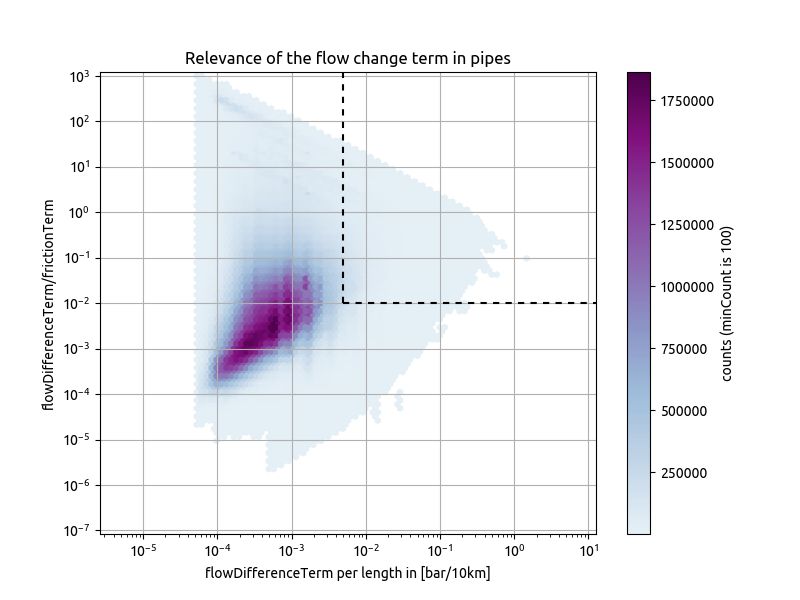
We plotted the results in Figure 1, using the normalized length |α|/10 km
and the friction value ratio |α|/|β| as axes. The dashed lines mark the relevance
thresholds, i.e., all points outside of the top right area do not have relevant α
values. For the length normalized α value, we will focus on points of small and
high relevance having a minimum value of 0.1 bar per 200 km, which translates
into a value of 0.005 bar per 10 km.
Figure 1 shows that most points are clustered in the area between α values
of 10−4 and 3 · 10−3 per 10 km and |α|/|β| ratios of 10−4 and 10−1 . Due to
5Figure 1: Hexagon plot of all data points having a flow change of at least
3
0.5 1000h m . The color of the hexagon represents the number of associated origi-
nal data points. The minimum count per hexagon is 100 (∼ 10−6 of all points).
The dashed lines mark the area of values fulfilling the two threshold criteria for
relevant points, i.e., all points outside of the marked top right area do not have
relevant α values.
the length normalized α threshold, all of these are not relevant for our ongoing
analysis. The diagonal line at the top right end of the point set indicates that
extreme values regarding the two threshold criteria do not coincide. Furthermore,
we assume that the point set’ straight-line boundary on the left side is caused by
the minimal flow change threshold applied in the analysis’ previous step.
In the following, we will continue to analyze those points fulfilling both rele-
vance criteria, which are roughly 21 million data points.
3.3 Inertia term on paths
In the previous steps, we have derived a set of pipe and time point combinations
that potentially have relevant absolute sizes of |α| by normalizing their α values
by the pipe length. In this step, we will now look at the actual absolute α values
produced by these data points.
First, we group the data points by time and look at each pair of subsequent
time points individually. For each of these pairs, we sort the data points into con-
nected components based on the corresponding pipes and the underlying network
topology. In each connected component, we determine the α-related absolute er-
ror as the length of a longest path in the component using the absolute α values
as lengths per pipe. The motivation for this procedure is the fact that the er-
ror caused by removing α from the momentum equation accumulates over space,
along the pipes of the network. In other words, the pressure difference of a path
of pipes connecting two active elements is the sum of pressure differences defined
by Equation (2), which includes the sum of corresponding α values for each of
the pipes.
6For creating the connected components, we group the pipes into sets connected
directly by sharing an endnode or indirectly via other pipes in the set, valves
being open at that point in time, or any resistors. We do not use the active
elements, i.e., regulators and compressor stations, to connect the pipes since we
are interested in the error on pipelines connecting these elements. As mentioned
above, the maximum error inside a component is determined as the weight of a
longest path when considering the absolute α values as edge weights. Note that
we use a directed graph as a representation of the connected component when
searching for a longest path. Each pipe is directed according to its topological
orientation for positive α values and against the topological orientation otherwise.
Open valves are added twice, once per orientation with a length value of zero. For
resistors, we are not guaranteed to have a flow value given in the data. However,
we can deduce the flow change from the pressure values of the endnodes: If the
pressure reduction along the resistor increased, the flow through the resistor did
so as well and we direct the arc according to its topological orientation. If it
decreased, we choose the opposite direction, and if it stayed the same, we add
arcs for both directions. In any of the cases, the weight of resistor arcs is zero.
An artificial example of a connected component with pipe flow values for a pair
of time points, corresponding α values, and the longest path determining the α
value for the whole component can be found in Figure 2.
Note that the directed variant of the longest path search is necessary to prevent
parallel loop lines in the component to count twice, i.e., once in both directions,
even though their flow change and the associated α values are oriented towards
the same node, see again Figure 2 for an example. To calculate the longest path
length, we search for a shortest path in the directed graph using negated weights
for all pipes and negate the final result. In the rare case of negative cycles, we
save the negative cycle length, set the length of all affected arcs to zero, and
add all negative cycle lengths to the final longest path length. Hence, we may
overestimate the length of the longest path and the connected component’s α
value.
When applying this procedure to the set of pipe and time point combinations,
we find 6.3 million connected components created from the 21 million different
data points. From these connected components, 79,000 contain a longest path
length in terms of absolute α values with length ≥ 0.1 bar and 2,500 have a path
length of at least 0.5 bar. In other words, a flow change causing an absolute α
value of more than 0.1 bar on a path between active elements occurs on average
every 23 minutes in the network. A corresponding flow change for an absolute α
value of at least 0.5 bar happens on average every 12 hours. In sum, 1.3 million
single pipe data points are contained in the components for 0.1 bar and 51,000
for 0.5 bar, or 0.036 % and 0.0014 % of all 3.6 billion data points, respectively. An
overview of the number of components and data points for different thresholds
can be found in Table 1.
3.4 Inertia term over time
The previous section’s results already indicate that α is indeed too small to be
relevant for the vast majority of cases. A connected component featuring highly
relevant α values on average only occurs in the network every 12 hours, or each
240th time step, or 2500 times in total. However, in this step of the analysis, we
740
200
40
80 80 240
640 560
80 40
120 720 240 80
1200 400
40 40
360 240
40 40
320 280
a) Network with flow value changes
0.01
0.02
0.05 0.04
0.06 0.02
0.0
0.09 0.0 0.03
0.0
0.03 0.02
0.03 0.02
b) Longest path in α value graph with total error value of 0.29
Figure 2: Example of finding a longest α value path in a connected component.
The upper Figure a) shows a connected component enclosed by active elements,
in which the numbers represent flow values for each pipe at the first point in time
(upper value) and the subsequent time point (lower value). The lower Figure
b) shows the directed arcs induced from the pipes, open valves, and resistors,
where the numbers represent the α values on each of the arcs. The longest
directed path regarding the α values represents the maximum error value in the
component. Note that the pure sum of all α values in the component, as well
as the undirected longest path in the component, would both overestimate the
component’s error value.
will have an even closer look at these remaining connected components and their
51,000 data points.
First, we determine how often in the 51,000 data points one pipe is contained
in a highly relevant connected component at two or more subsequent time points.
If this is not the case, then the errors made by not including the α value in the
pipe equation appear only for a brief period of time, i.e., that point in time in
which the flow value changes to a different level. More importantly, the α value
errors decrease if we would increase the time granularity to more than 3 minutes.
In the literature on transient gas network optimization, the time step size usually
ranges from 5 to 10 minutes, as in Mak et al. [2016], Burlacu et al. [2019], to
whole hours, like in Moritz [2007], Domschke et al. [2011], Zlotnik et al. [2015]. If
the α value is caused by a single large change in the flow values, its value would
decrease by a factor of more than 3 for a 10 minute time granularity.
8Threshold # Components # Contained Pipes avg comp occurance
0.1 bar 79,000 1,300,000 1 every 23 minutes
0.2 bar 19,000 370,000 1 every 1.6 hours
0.3 bar 7,500 150,000 1 every 4.0 hours
0.4 bar 3,900 81,000 1 every 7.7 hours
0.5 bar 2,500 51,000 1 every 12 hours
0.6 bar 1,700 35,000 1 every 18 hours
0.7 bar 1,200 26,000 1 every 25 hours
0.8 bar 930 20,000 1 every 1.3 days
0.9 bar 720 16,000 1 every 1.7 days
1.0 bar 580 13,000 1 every 2.2 days
Table 1: Overview of connected component statistics for different thresholds of
the absolute α value on a longest path in the component. For each threshold,
we give the number of components having a longest path length of at least the
given value and the sum of all pipe data points over all these components. In
addition we give the average component occurance, determined from the number
of components and the number of overall time steps. All Numbers are rounded
to 2 significant digits.
In our data, 92 % of the 51,000 data points have not been in connected compo-
nents with high α values for more than one consecutive time step. Less than 6 %
of the data points appear in connected components two times in a row, and less
than 2 % of points in three components in a row. The longest series of time points
for a single pipe in a connected component with highly relevant α values was 8. In
total, there are only 8,700 out of the 51,000 data points for which the pipe is in a
connected component of highly relevant α value also for the previous or next time
interval. These data points are contained in 570 different connected components
in total. Since we count a connected component per single time point, there are
at most 285 consecutive time point series of length at least 2 having intersecting
connected components of high α values. Hence, these appear on average every
4.4 days.
3.5 High flow change values
As the final part of our analysis, we look at the size of absolute flow value changes
in single data points. From the formula (3) for α follows that it increases in abso-
lute terms with an increasing absolute flow value difference |Q0t1 − Q0t0 |. However,
at a certain size, the flow changes are considered to be unrealistically high. These
values can occur in a simulation-like process like the one the data was generated
with but are too large for real-world operating conditions. Flow changes like these
would put much strain on the single network elements, make the general network
situation unstable, and cause a lot of noise, which all is not desirable from a
network operator’s point of view. Therefore, there are elements to prohibit these
large gas flow changes, for example, by slowly synchronize the pressure levels of
two pipelines, which operated separately before and should now be connected.
For our analysis, we choose a rather high value of ∆real 3
Q0 = 2, 000, 000 m /hour
to be the limit for realistic flow value changes during a 3 minute time period.
This is roughly equal to the absolute size of the network’s biggest entry being
9shutdown from maximum flow to zero during a 3 minutes time period. Note that
this value should actually be much smaller for pipes with smaller diameters since
the corresponding velocity of the gas and hence also its noise level is higher for
the same amount of flow.
From the 2,500 connected components of high relevance, roughly 800 contain a
pipeline whose absolute flow change exceeds ∆real
Q0 . The remaining 1,700 connected
components contain roughly 37,000 single data points. If we repeated the time
point series analysis from the previous Section 3.4based on this reduced set of
values, we find 4,400 data points in time point series of length at least two. The
longest time series are of length 4, i.e., present over 12 minutes, and all data
points are contained in 240 connected components. Therefore, there are at most
120 consecutive time point series of length at least 2 having intersecting connected
components of high α values. Hence, they appear on average every 10.4 days. We
consider this final average appearance rate of high relevant α values large enough
to verify that α can be removed from the momentum equation since it is mostly
irrelevant in realistic flow scenarios.
As a final remark, we want to highlight that after high-value flow changes,
some parts of the change are often taken back during the following time steps.
This means that the flow stabilizes at some level, which is much closer to the orig-
inal flow value than the one producing the large initial flow change value. We did
not quantify this effect, but when having unrealistically large flow changes, the
following changes in the opposite direction can produce α high relevance values as
well. For example, we found out that every time series of length bigger than 5, pro-
duced from the set of 51,000 data points including the flow change value over ∆real
Q0 ,
originates from two flow changes of 2,000,000 m3 /hour and 10,000,000 m3 /hour
at one point in time and the following flow changes into the opposite direction
during the subsequent time points. These changes happening after the initial
huge flow change would also be avoided in reality by reducing the size of the ini-
tial flow change and, therefore, further reducing the number of occurring network
situations with relevant α values. Having longer time steps would also reduce
the α value in these situations since the initial flow changes are reduced by the
following smaller changes in the opposite direction.
4 Summary
In this article, we evaluated the size of the inertia term α in the momentum
equation on a large set of real-world gas network state data over a consecutive
period of 41 months to review the statement that α is small and negligible under
realistic operation conditions. After establishing thresholds defining the relevant
absolute sizes of the term and the relevant sizes of the term in relation to the
friction value, we analyzed the data in multiple steps: After reducing the number
of data points to consider by sorting out those having a too-small flow change
value, we found those data points for single pipes and time point pairs that
have the potential to lead to relevant values of α when scaled to the maximum
distance between active elements of 200 km. In the next step, we grouped these
values by time and into connected components based on the network topology.
In these components, we established the overall absolute α value as the length of
a longest directed path in terms of α values. Components with highly relevant α
10values determined by this method occur on average every 12 hours in the network.
Finally, we determined those components in this set, which persist over more than
a single 3-minute time step and do not feature unrealistically high flow values.
We found that there are only 120 of these components in the network during the
entire time horizon, each lasting at most 12 minutes. Hence they only appear less
often than once every 10 days. Therefore, we conclude that network situations
featuring high relevant α values are rare enough to discard α from the momentum
equation without losing much accuracy.
Acknowledgements
The work for this article has been conducted in the Research Campus MODAL
funded by the German Federal Ministry of Education and Research (BMBF)
(fund numbers 05M14ZAM & 05M20ZBM).
References
Jens Brouwer, Ingenuin Gasser, and Michael Herty. Gas pipeline models re-
visited: Model hierarchies, nonisothermal models, and simulations of net-
works. Multiscale Modeling & Simulation, 9(2):601–623, 2011. doi: https:
//doi.org/10.1137/100813580.
Robert Burlacu, Herbert Egger, Martin Groß, Alexander Martin, Marc Pfetsch,
Lars Schewe, Mathias Sirvent, and Martin Skutella. Maximizing the storage
capacity of gas networks: A global MINLP approach. Optimization and Engi-
neering, 20(2):543–573, June 2019. doi: 10.1007/s11081-018-9414-5.
Günther Cerbe. Grundlagen der Gastechnik: Gasbeschaffung - Gasverteilung -
Gasverwendung. Carl Hanser Verlag GmbH & Co. KG, seventh edition, April
2008. ISBN 978-3-446-41352-8.
Ning Hsing Chen. An explicit equation for friction factor in pipe. Industrial
& Engineering Chemistry Fundamentals, 18(3):296–297, 1979. doi: 10.1021/
i160071a019.
Pia Domschke, Björn Geißler, Oliver Kolb, Jens Lang, Alexander Martin, and
Antonio Morsi. Combination of Nonlinear and Linear Optimization of Transient
Gas Networks. INFORMS Journal on Computing, 23(4):605–617, 2011.
Pia Domschke, Benjamin Hiller, Jens Lang, and Caren Tischendorf. Modellierung
von Gasnetzwerken: Eine Übersicht. 2017.
Klaus Ehrhardt and Marc C. Steinbach. Nonlinear Optimization in Gas Networks.
In Modeling, Simulation and Optimization of Complex Processes, pages 139–
148. Springer, Berlin, Heidelberg, 2005.
A.E. Fincham and M.H. Goldwater. Simulation models for gas transmission net-
works. Transactions of the Institute of Measurement and Control, 1(1):3–13,
1979. doi: 10.1177/014233127900100101.
11M. Herty, J. Mohring, and V. Sachers. A new model for gas flow in pipe networks.
Mathematical Methods in the Applied Sciences, 33(7):845–855, 2010. ISSN 1099-
1476. doi: 10.1002/mma.1197.
Terrence WK Mak, Pascal Van Hentenryck, Anatoly Zlotnik, Hassan Hijazi, and
Russell Bent. Efficient dynamic compressor optimization in natural gas trans-
mission systems. In American Control Conference (ACC), 2016, pages 7484–
7491. IEEE, 2016. doi: 10.1109/ACC.2016.7526855.
Susanne Moritz. A Mixed Integer Approach for the Transient Case of Gas Net-
work Optimization. PhD thesis, Technische Universität Darmstadt, Darmstadt,
2007.
OGE. Open Grid Europe GmbH. https://oge.net.
Andrej J. Osiadacz. Different Transient Flow Models - Limitations, Advantages,
And Disadvantages. In PSIG-9606. Pipeline Simulation Interest Group, 1996.
Papay. A termeléstechnológiai paraméterek változása a gáztelepek muvelése
során. OGIL Musz. Tud. Kozl., 1968.
Jamal M Saleh. Fluid Flow Handbook. McGraw-Hill Professional, 2002.
J. F. Wilkinson, D. V. Holliday, E. H. Batey, and K. W. Hannah. Transient Flow
in Natural Gas Transmission Systems. American Gas Association, 1964.
Anatoly Zlotnik, Michael Chertkov, and Scott Backhaus. Optimal control of
transient flow in natural gas networks. In 54th IEEE Conference on Decision
and Control (CDC), pages 4563–4570. IEEE, 2015. doi: 10.1109/CDC.2015.
7402932.
12You can also read