FB-MULTIPIER Step-By-Step Advanced Example Problems
←
→
Page content transcription
If your browser does not render page correctly, please read the page content below
FB-MULTIPIER
         Step-By-Step Advanced Example Problems

     March 2005

1.
MP-1. BRIDGE OVER WATER MODEL

        Shown in Figure 1.1 is a two-span portion of a six-span bridge, which will be modeled in

Example MP-1. The bridge spans a navigable waterway crossing, where the piers are subjected to axial

loads and a potential lateral vessel collision load. In addition to dead load and a vessel collision load, the

bridge will be subjected to vehicular live loads and wind loads. Loads will be applied and combined using

the AASHTO LRFD Design Specification. This example builds upon the pier modeled in Example 2 in

the FB-Pier Users Manual. The user is encouraged to review single pier modeling examples before

modeling a full bridge using FB-MultiPier.

                                                                                           100 ft

                                                          150 ft

                        Figure 1.1 Example MP-1, Two-Span Bridge Structure

FB-MULTIPIER USERS MANUAL                                                                                 1-2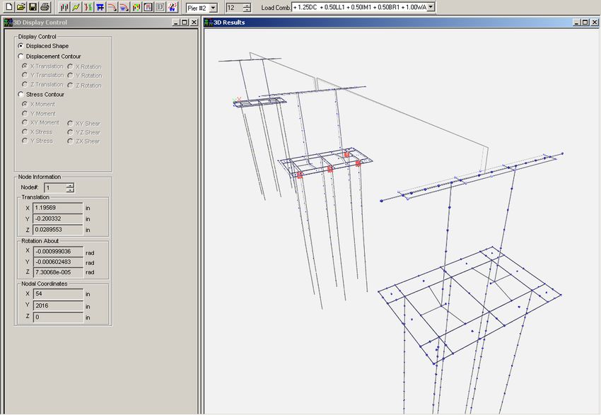
To recap, the pier modeled in Example 2 consists of 6-54 inch drilled shafts (80 ft long) and two

pier columns which are 30 ft tall, 5 ft square and spaced 16 ft apart. The pier cap is 4 ft thick and the

drilled shaft cap is 10 ft thick with a 4.5 ft overhang. Due to scour, the sand surface is located 15 ft below

mean sea level, and the soft rock is characterized as FHWA's intermediate geomaterial. The properties of

the sand and rock are given in Figure 1.2. This pier model will be used to support the two spans modeled

in this bridge example.

                                    150 kips         250 kips         150 kips

                                                                       14’
                                         10’            16'
                                                                                  30'

                     1000 kips

                              15'
                                                                                 Water

                       Sand                    80'                           N = 35
                       γt = 120 pcf                             35'          k = 150 pci

                                                                             Cu=2.8ksi
                          Soft Rock,
                                                                             qt=0.28ksi
                          γt = 140 pcf
                                                                             ε50 = 1%

                                     Figure 1.2 Example 2, Pier Structure

        This example will consider AASHTO LRFD design load combinations to determine the worst

case loading scenario for the drilled shafts and pier. The following LRFD limit states will be checked:

        STRENGTH-I, STRENGTH-III, STRENGTH-V, EXTREME-II, SERVICE-I

FB-MULTIPIER USERS MANUAL                                                                                 1-3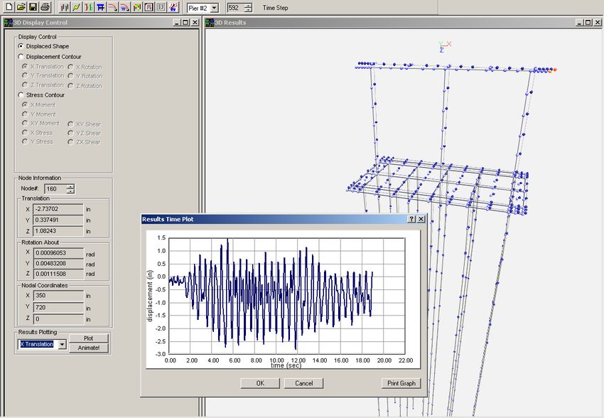
The load types shown below in Table 1.1 will be considered. The bearing loads shown in the

table result from a live load placed on Span #1. The “(L)” marker indicates that the load will be applied in

the left bearing row. Each pier has two rows of bearings.

  Dead Load (DC)                 Automatically generated by the program (self weight)

  Water Load (WA)                Automatically generated by the program (buoyancy)

  Live Load (LL1)                Bearing 1 (L)    80 kips
                                 Bearing 2 (L)    120 kips
                                 Bearing 3 (L)    0 kips          Vehicular Live Load
                                 Bearing 4 (L)    0 kips

  Impact Load (IM1)              Bearing 1 (L)    26 kips
                                 Bearing 2 (L)    40 kips
                                 Bearing 3 (L)    0 kips          Vehicular Dynamic Load Allowance
                                 Bearing 4 (L)    0 kips

  Braking Load (BR1)             Bearing 1 (L)    15 kips
                                 Bearing 2 (L)    15 kips
                                 Bearing 3 (L)    15 kips         Y-direction (longitudinal) load
                                 Bearing 4 (L)    15 kips

  Live Load (LL2)                Bearing 1 (L)    100 kips
                                 Bearing 2 (L)    110 kips
                                 Bearing 3 (L)    105 kips        Vehicular Live Load
                                 Bearing 4 (L)    0 kips

  Impact Load (IM2)              Bearing 1 (L)    33 kips
                                 Bearing 2 (L)    36 kips
                                 Bearing 3 (L)    35 kips         Vehicular Dynamic Load Allowance
                                 Bearing 4 (L)    0 kips

  Braking Load (BR2)             Bearing 1 (L)    20 kips
                                 Bearing 2 (L)    20 kips         Y-direction (longitudinal) load
                                 Bearing 3 (L)    20 kips
                                 Bearing 4 (L)    20 kips

  Wind Load on Structure (WS)    To be generated using wind angles of 0, 30, and 60 degrees

  Wind Load on Live Load (WL) To be generated using wind angles of 0, 30, and 60 degrees

  Vessel Collision (CV)          Node 38          1000 kips         (Lateral - Applied to center of pile cap)

                                Table 1.1 Loads Applied to Bridge Model

Select Open from the File menu and choose Example2.in from the program directory (Figure 1.3).

FB-MULTIPIER USERS MANUAL                                                                                       1-4
Figure 1.3 Example2.in Model View

        The layout of the screens in the FB-MultiPier program is similar to that of FB-Pier to provide a

smooth transition between programs. New to FB-MultiPier, however, is the Model Data tree view that

allows for easy navigation between the data pages. This navigation can be achieved by using the mouse

or by using the arrow keys or the Ctrl-tab key combination. The tree items shown in light grey are either

not available for the current model type or can be enabled if certain modeling options are selected.

        The first step in modeling the bridge is to modify the single pier that will ultimately be used as a

template when generating more piers. The single pier in Example 2 contains concentrated loads applied

along the pier cap and a concentrated lateral load applied at the pile cap. The pier cap loads will be

replaced by a superstructure dead loads and wind loads generated by the program. The concentrated

FB-MULTIPIER USERS MANUAL                                                                               1-5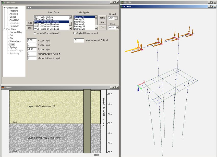
lateral load will only be applied to one of the three piers to simulate vessel collision. To delete the current

loads, select the Load data page in the Model Data window and click the “Del” to the left of the load case

list. After doing so, only a placeholder for a Preload case will remain. The bridge spring applied to the

pier cap should also be removed. When analyzing single piers, a bridge spring is typically used to model

the lateral stiffness of the superstructure. This spring is no longer needed since the full bridge model will

incorporate the superstructure. To delete the bridge spring, select the Springs data page in the Model Data

window and click the “Del” button. The pier can now be used to generate a complete bridge model.

        The next step in modeling the bridge is to provide bearing locations on the pier cap for the bridge

girders. To specify bearing locations, click on the Pier item in the Model Data tree view and then click

the “Use Bearing Locs.” button to enable bearing location modeling. Click on the “Bearing Locs.” button

to enter the bearing data. A single bearing row is modeled by default. Select “Two Rows” for the Bearing

Layout. Enter the values shown in the Left Bearing Row and Right Bearing Row Group in Figure 1.4.

FB-MULTIPIER USERS MANUAL                                                                                  1-6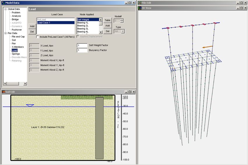
Figure 1.4 Bearing Locations

        Bearing locations can be modeled using a uniform or variable spacing. This example calls for 4

bearing locations at a Uniform spacing of 12 ft, offset -10 ft from the first column. The bearings will be

offset 1.5 ft from the centerline of the pier cap. In order to establish a naming convention, bridge spans

are assumed to be modeled in the positive ‘y’ direction. In doing so, the first row of bearings is called the

“Left Row” and the second row of bearings is called the “Right Row.” It is important to note that bearings

in the left and right rows do not have to coincide (although they do in this example). That is, there can be

a bearing in one row without a corresponding bearing in the other row. This capability allows for more

flexibility in laying out the girder locations on the pier.

        The pier model, now with bearings, will be used generate the two remaining piers for this

example. Before doing so, however, the model must first be converted to a Bridge model type (the model

is currently a General Pier model). To do so, click on the Problem data page and select the “Bridge”

Problem Type and confirm the intended model transformation by clicking “Ok” at the dialog prompt. FB-

MultiPier automatically generates a single bridge span and a matching pier at the end of the bridge span.

The bridge model is shown in a Plan View and 3D View in Figure 1.5.

FB-MULTIPIER USERS MANUAL                                                                                1-7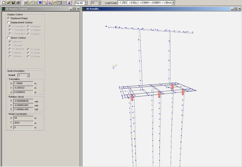
Figure 1.5 Single Span Bridge Model

        FB-MultiPier models a bridge span using an equivalent beam element with section properties that

represent the actual span. The span element connects to the bearing locations using rigid links in order to

transfer the load from the superstructure to the pier. The span element properties will be modified shortly.

        The pier generation and bridge layout capabilities are located in the Bridge data page. Select the

“Bridge” item in the Model data tree view to view this page. Figure 1.6 shows the options available for

modeling a bridge. The page is divided into model data for the Substructure (the pier foundation) and the

Superstructure (the bridge span).

FB-MULTIPIER USERS MANUAL                                                                               1-8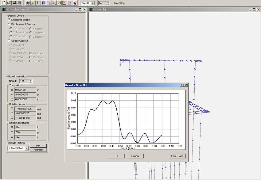
Figure 1.6 Bridge Data Page

        In the Substructure group, the Substructure combo box allows the user to select a pier for editing.

The Model Type combo box allows the user to select either a General Pier or Pile Bent model type for the

current pier. The Global X and Y Coordinates are used to position the pier model and the Rotation Angle

is used for rotating the pier about the vertical (global-Z) axis. Pier rotation is typically used in curved

alignments or skewed bridges. The Continuous Span option models span continuity over a pier support.

The Bearing Row Support Conditions allows for either One Row or Two Rows of bearings.

        Clicking the “Edit Supports” button allows the user to verify and/or modify the boundary

conditions at the bearing locations as shown in Figure 1.7. The Left/Right Bearing Row combo boxes

allow the user to specify a pre-defined boundary condition for the bearing row. The program provides

options for a Roller, Pin, Integral, or Custom boundary condition for each bearing row. Bearing rows at

the beginning and end of the bridge are given the “N/A” designation because there are no girders

associated with these bearing rows. Select a “Roller” Support Condition for the Right Bearing Row.

Notice that each bearing direction in the Right Bearing Row has a “Constrain” boundary condition except

FB-MULTIPIER USERS MANUAL                                                                              1-9
for the Y-translation and the rotation about the X-axis (RX), which have a “Release” condition. This
combination of boundary conditions models a roller connection at the first pier.
Figure 1.7 Custom Bearing Connection
Although not used in this example, custom boundary conditions can be entered by clicking the
“Edit Custom Bearings” button. Custom boundary conditions are described using a load-displacement
curve and can be applied to one or more bearing directions. Click “Ok” to close the Custom Bearing
Connection dialog.
In the Superstructure group, the Span combo box allows the user to select a bridge span for
editing. The “C/C Length” box shows the center-to-center length for the span (measured from the center
of the right bearing row to the center of the left bearing row on the next pier). Click the “Edit Span”
button to modify the bridge span properties. Enter the values shown in Figure 1.8.
FB-MULTIPIER USERS MANUAL 1-10Figure 1.8 Bridge Span Properties
The Bridge Span Properties dialog is divided into two types of data input. The Section Properties
group refers to the flexural properties of the equivalent bridge span element. The properties can either be
constant or variable along the span. A table is provided for entering variable properties for the 10 equal-
length elements along the span. The values enter in the Section Properties group reflect the entire bridge
cross-section (i.e. girders, slab, parapets, etc.). Note that the values shown are for demonstration purposes
and do not reflect values used in a specific bridge design. The Span Profile Properties group is used
described the profile and height of the span. The Transverse Area is the exposed span area that will be
used in the wind load application to the structure. The Begin Height and End Height are used to model the
equivalent span element through the center of gravity of the span. These values are measure from the
center of gravity of the pier cap to the center of gravity of the span. The Live Load Height is used in
generating wind on live load cases. Click “Ok” to apply the values and return to the Bridge data page.
Bridge spans automatically connect one pier to the next. Therefore, to change the span length, the
user must change the global coordinates of the pier. In the Bridge data page, first select “Pier 2” from the
FB-MULTIPIER USERS MANUAL 1-11Substructure combo box and then change the Global Y Coordinate from 100 ft to 150 ft to reflect the span
length for this example. Click the “Edit Supports” button and select “Pin” for the Left Bearing Row in the
Custom Bearing Connections dialog. Click “Ok” to apply the changes. The updated bridge model is
shown in Figure 1.9. Note that the center to center span length is displayed as 147 ft since the span is
measured from the bearing centerlines and not the center of the pier cap. Also note that the equivalent
span element is modeled above the pier cap based on the center of gravity heights specified in the Bridge
Span Properties dialog.
One more pier must be added to the model in order to complete the bridge generation process. To
do so, select “Add Pier” from the Substructure combo box. A dialog will appear that gives options for the
new pier. Select the Structure Type “General Pier” and select Pier 2 from the “Select Model” menu. A
duplicate of pier 2 will automatically be generated and positioned based on the previous span length. This
example calls for a span length of 100 ft for the second span. Enter 250 ft for the Global Y Coordinate for
Pier 3. The updated two-span bridge model is shown in Figure 1.10.
This example calls for a continuous span over the middle pier. Select “Pier 2” from the list of
substructures in the Bridge data page. Check the “Continuous Span” checkbox to model span continuity
over Pier 2. This option will allow the internal bending moment to transfer between bridge spans. Notice
that the span continuity option is not available for Pier 1 or Pier 3 because these piers are at the ends of
the bridge. Span continuity can be verified by inspecting the span over a pier support in the 3D Bridge
View window. The span line will be unbroken if span continuity is modeled.
FB-MULTIPIER USERS MANUAL 1-12Figure 1.9 Increased Bridge Span
Figure 1.10 Two Span Bridge Model
FB-MULTIPIER USERS MANUAL 1-13Several bridge span and bearing details must be updated before the model is complete. First,
select “Span 2” from the Span combo box in the Superstructure group. Click the “Edit Span” button and
change the Transverse Area to “1000” ft2 in the Bridge Span Properties dialog since the span is only 100
ft long. Click “Ok” to apply the properties. Second, in the Substructure Group, Pier #3, change the
Bearing Row Support Conditions to “Roller” for the Left row. Note that the bearing conditions for the
Pier #2 are set at “Integral” for both the Left and Right rows. Change both bearing rows in Pier #2 to
“Pin.”
Now that the bridge model has been created, it is easy to apply load cases to the full bridge. In
this example, AASHTO LRFD load combinations will be used to determine the governing loads for the
bridge. To begin, select the Analysis data page in the Model Data window and then check the “AASHTO
Combinations” check box as shown in Figure 1.11. Doing so will enabled AASHTO load combination
capabilities for the entire bridge.
Figure 1.11 Analysis Data Page – Enabling AASHTO Load Combinations
FB-MULTIPIER USERS MANUAL 1-14AASHTO load cases are managed using the AASHTO data page. Select this page to view the
various loading option, as shown in Figure 1.12. The AASHTO Load Factors group allows the use to edit
the load factors used in the load combination equations. This can be done for either an LRFD analysis or
an LFD analysis. The Limit States to Check group is used to specify which limit states to consider in the
analysis as well as whether to reverse the loads and check maximum/minimum load factors (LRFD only).
Finally, the Automated AASHTO Loads group is used to specify the types of loads to consider in the
analysis. A Load Case Manager is provided in this group to add, modify, or delete AASHTO load cases
for the model. This group also includes options for automatic generation of self weight, buoyancy, and
wind load cases.
Clicking the “Load Case Manager” displays the AASHTO Load Manager dialog (Figure 1.13).
The dialog shows the AASHTO load types that are available and the load types are currently defined for
the model. Initially, the “Defined Load Cases” list is empty as no AASHTO load types have been added
to the model in this example.
Figure 1.12 AASHTO Data Page
FB-MULTIPIER USERS MANUAL 1-15Figure 1.13 AASHTO Load Case Manager
This example will consider a simple bridge loading consisting of dead (self weight and
buoyancy), live, and wind loads. Load cases are added to the model by selecting a load case from the
“Available Types” list and then clicking the “Several observations can be made at this point. First, some load case types can have multiple load
cases. These types have the number of currently defined load cases shown in parenthesis. Multiple load
cases are enabled for live loads and wind loads. To change the number of load cases defined for a given
load type, enter a new value in the box shown below the Defined Load Cases list. Second, certain loads
are automatically generation based on the existence of either live loads or wind loads. For live loads,
Impact and Vehicle Braking cases are automatically included with the live load. For wind loads, Wind
Load on Structure and Wind Load on Live Load are added in tandem. Finally, when the number of live
loads is changed, the number of Impact and Vehicle Braking cases is automatically updated. The same is
true for wind load cases.
This example will consider the effect of 2 live load cases and 3 wind load cases. Click on the
“Live Load” item in the Defined Load Cases list. Enter 2 in the edit box to change the number of live (and
impact and braking) cases to 2. Next, click on the “Wind on Structure” item in the Defined Load Cases
list and enter 3 in the edit box to change the number of wind load cases. The resulting screen is shown in
Figure 1.15.
Figure 1.15 AASHTO Load Case Manager – Multiple Load Cases
FB-MULTIPIER USERS MANUAL 1-17After defining the load case types for the model, the loads can then be applied to the entire bridge.
Click Ok to process the load changes to the model. A dialog will be displayed (Figure 1.16) to inform the
use of the changes that will be made to the model. This summary window is important and requires the
user to confirm the changes made to the model. Clicking “Yes” will modify the load cases for the entire
bridge. Clicking “No” will abandon the proposed load case modifications and return the user to the
AASHTO Load Manager. For this example, click “Yes” to confirm the changes and apply the load types
to the entire bridge.
Figure 1.16 Confirming Load Case Modification for Entire Bridge
In addition to synchronizing the load types for all piers in the model, the AASHTO Load
Manager also ensures that concentrated load placeholders are created at the bearing locations to
accommodate loads applied from the superstructure. In this example, all of the defined load types except
for the “Water Load” and “Vessel Collision” type, are expected to have loads applied at the bearing
locations. The Dead Load of Components (self weight) is applied internally; therefore, no additional load
needs to be applied to the bearings. The concentrated load placeholders are still provided; however, in
case the user wishes to apply additional load. Wind loads will be automatically applied to the pier
FB-MULTIPIER USERS MANUAL 1-18bearings using the Wind Load Generator on the AASHTO data page. The live loads will manually be
applied to the bearing locations since the program does not currently contain a live load generator. The
vessel collision load will be manually applied to the pier as well.
Wind Loads
As stated, FB-MultiPier can automatically apply wind loads to the entire bridge using the
AASHTO Wind Load Generator. This can be done by clicking the “Wind Load Generator” button. This
example will consider 3 wind load cases, with wind applied at 0, 30, and 60 degrees. Specify “3” for the
Number of Cases and select “0”, “30”, and “60” for the wind angles as shown in Figure 1.17. The table
of wind pressures shows the default values given in the AASHTO LRFD code. These values should be
modified if necessary. Click the “Generate Wind Load Cases” button to apply the wind to the bridge and
transfer the loads to the pier bearings. Click “Yes” and then “Ok” to confirm the wind load case
generation.
Figure 1.17 AASHTO Wind Load Generator
Before proceeding to the remaining load types, it is important to brief discuss the methodology
used by the Wind Load Generator. As Figure 1.17 demonstrates, a uniform distributed load is applied
FB-MULTIPIER USERS MANUAL 1-19perpendicular to each span for Wind Load on Structure cases. The magnitude of this load is based on the
span profile area and the wind pressures in the Wind Pressures table and spans are assumed to be simply
supported when applying the uniform load. A line load is also applied perpendicular to the each span for
the Wind Load on Live Load cases. The magnitude of this load is based on the span length and wind
pressures in the Wind Pressures table. Both the Wind Load on Structure and Wind Load on Live Load are
applied at the center of gravity of the superstructure (as defined in the Bridge Span Properties dialog –
Figure 1.8). A wind load is also applied to the pier using the cross-section properties of the pier column
and pier cap and the wind pressures in the Wind Pressures table. All of the wind loads on the bridge are
transformed into concentrated loads acting at the bearing locations for each pier. This can be confirmed
by viewing the loads generated for the wind load cases. Note that only the generated wind loads are
shown as bearing loads at the piers. Figure 1.18 shows the wind loads generated at Pier #2 for the zero
wind angle case.
Figure 1.18 Wind Loads on Pier #2, 0o Wind Angle
FB-MULTIPIER USERS MANUAL 1-20Live Loads
Live loads can be applied to the pier using the Load data page. The user can either select each live
load case from the Load Case list or click on “Table” button to enter the loads in a spreadsheet format.
Table 1.2 provides the Live Load, Impact, and Vehicle Braking loads used in this example. These loads
are applied to the interior pier support (Pier #2). Similar loads could also be applied to the other piers and
is left as an exercise to the user.
Bearing Live Load (kip) Impact (kip) Braking (kip)
(Force Z) (Force Z) (Force Y)
(Case 1 – One Lanes Loaded)
1L 120 40 15
2L 80 26 15
3L 0 0 15
4L 0 0 15
(Case 2 – Two Lanes Loaded)
1L 100 33 20
2L 110 36 20
3L 105 35 20
4L 0 0 20
Table 1.2 Live Load, Impact, Braking
Select the Load data page in order to begin entering the live load data. Next, select “Pier #2” from
the pier selection combo box in the toolbar. The AASHTO Load Table provides a quick method for
entering the data if it is already in a tabular format. Click the “Table” button to view all load case data.
First, verify that the list cases listed in the AASHTO Load Table match the load cases generated using the
AASHTO Load Manager. After doing so, click on the “+” to expand and modify the load case “Live
Load 1”. Enter the live loads as shown in Figure 1.19. Next, enter the data given in Table 1.2 for Live
Load 2 and the Impact and Vehicle Braking load cases. Note that the Live Load and Impact cases have
vertical loads and the Vehicle Braking cases have horizontal (longitudinal) loads. The final AASHTO
Load Table is shown in Figure 1.20. Two additional items are worth mentioning. First, the Wind on
Structure and Wind on Live Load cases can be examined in this table to verify the results of the
AASHTO Wind Load Generator. Second, the Load Types list on the right side of the dialog is grayed out.
FB-MULTIPIER USERS MANUAL 1-21This list is only accessible for single pier problems. For full bridge problems, the AASHTO Load
Manager must be used to add and remove load cases.
Figure 1.19 AASHTO Load Table – Live Loads
Figure 1.20 AASHTO Load Table – Live Load, Impact, Vehicle Braking
FB-MULTIPIER USERS MANUAL 1-22Vessel Collision Load
The vessel collision load value can also be specified in the AASHTO Load Table. Scroll down to
the bottom of the table and expand the “Vessel Collision” load case. A default placeholder called “Node
1” is provided. Click on this placeholder to edit the node number. Change the number “1” to “38” to
apply the vessel collision load at Node 38 (center of the pile cap). Enter “1000” kips for the Force X as
shown in Figure 1.21. Note that although not demonstrated in this example, more concentrated loads can
be added by clicking the “Figure 1.22 AASHTO Limit States
The AASHTO data page automatically updates the Number of Load Combinations count as the
user selects Limit States to consider in the analysis. As shown in Figure 1.22, the current model analysis
will consider 19 load combinations. The equations for each of these combinations can be previewed in
advance of the analysis by clicking the “Preview Load Combinations” button. Figure 1.23 shows the
current load combinations.
Figure 1.23 Load Combination Preview
FB-MULTIPIER USERS MANUAL 1-24This completes the modeling phase for the bridge. To analyze the model under the applied loads,
click the (Analyze) button in the toolbar.
Results can be viewed after reaching a converged solution to the problem. Results are presented
per pier and the pier selection combo box in the toolbar is used to switch between piers. Click the
(Pile Results) button to view the maximum results for the piles. The pile group for the interior pier
support is of particular interest since it has the live load application at the support. Select “Pier #2” from
the pier selection combo box in the toolbar to view the results for the interior pier. The load combinations
with the vessel collision load are most likely to produce the maximum results. On this assumption, select
“EXTREME-II” from the limit state combo box in the Plot Display Control window. This will highlight
the pile with the maximum demand/capacity ratio and show the force results for the governing load
combination in the EXTREME-II limit state. The resulting plots are shown in Figure 1.24.
Figure 1.24 Maximum Pile Results – EXTREME-II
FB-MULTIPIER USERS MANUAL 1-25To view the pier column results, click the (Pier Results) button. The limit state combo box
can again be used determine the maximum load combination result for each limit state. In this example,
the EXTREME-II limit state has the maximum demand/capacity ratio for the pier columns, although not
by much. The other limit states have similar results. This is due to the fact that the vessel collision load is
applied at the pile cap, so most of the load transfers into the foundation and not into the pier columns. The
resulting plots are shown in Figure 1.25.
Figure 1.25 Maximum Pier Column Results – EXTREME-II
The deformed shape of the pier and bridge model can provide additional insight into the model
behavior. Click the (3D Results) button to view the deformed shape for Pier #2. The deformed pier is
shown in Figure 1.26. Note that the red markers at the pile heads indicate plastic hinging zones. The pile
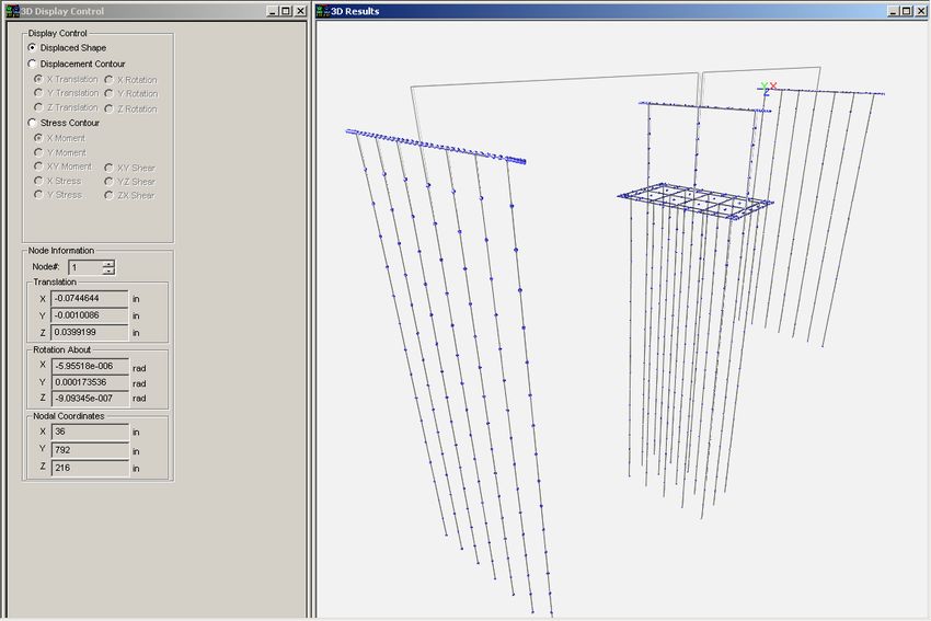
capacity has been exceeded at these plastic hinge zones. Right-clicking the mouse in the 3D Results
FB-MULTIPIER USERS MANUAL 1-26window and selecting “Bridge View” from the popup menu will show the 3D view of deformed shape for
the entire bridge. This view is shown in Figure 1.27.
Figure 1.26 Pier #2 Deformed Shape – EXTREME-II
FB-MULTIPIER USERS MANUAL 1-27Figure 1.27 Bridge Deformed Shape – EXTREME-II
This concludes Example MP-1.
FB-MULTIPIER USERS MANUAL 1-28MP-2. HIGHWAY OVERPASS BRIDGE MODEL
Shown in Figure 2.1 is a two-span highway overpass bridge, which will be modeled in Example
MP-2. The bridge is supported by pile bent abutments and a general pier interior support. The bridge is
primarily subjected to vertical loads, but there is some concern about a possible vehicle collision force on
one of the columns in the pier. The default Bridge model type will be used in creating the bridge model
for this example.
Collision
force
60 ft
60 ft
Figure 2.1 Example MP-2, Two-Span Highway Overpass Structure
FB-MULTIPIER USERS MANUAL 1-29Select New from the File menu and choose Bridge (Multiple Piers) from the New Problem Type
screen as shown in Figure 2.2 and click “Ok”. The program will provide a default single-span Bridge
model, as shown in Figure 2.3.
Figure 2.2 Example MP-2, Two-Span Highway Overpass Structure
FB-MULTIPIER USERS MANUAL 1-30Figure 2.3 Default Bridge Model
The bridge in this model consists of two pile bent abutments and a general pier interior support.
To convert the first pier to a pile bent, click on the Bridge data page in the Model Data window. The first
pier is automatically selected as the active pier. Select “Pile Bent” from the Model Type combo box to
change the pier to a pile bent. Click “Ok” to confirm the model transformation. Select “Default Pile Bent”
when prompted to Select Model. The resulting model type transformation looks a little unusual in the 3D
Bridge view window at first because the bent cap and pier cap elevations are not the same. Also note that
the span has been removed because the number of bearing locations do not match. This will be corrected
shortly. To create the third pier, select “Add Pier” from the Substructure combo box. In the Substructure
dialog that appears select “Pile Bent” for structure type and “Pier 1 Bent” from the Model type menu.
The program will automatically copy the pier data from the first pier to the third pier. Note that when
adding a pier, the new pier automatically becomes the active pier. To change the currently selected (third)
FB-MULTIPIER USERS MANUAL 1-31pier to a pile bent model type, select “Pile Bent” from the Model Type combo box. The resulting changes
are shown in Figure 2.4.
Figure 2.4 Bridge Model with Pile Bent Abutments
The next step in the bridge modeling is to adjust the elevations of each foundation to model a
level bridge span. This can be accomplished by changing the elevation of the interior pier support (or by
changing the elevations of the abutments). To do so, select “Pier 2” from the Substructure combo box in
the Bridge data page. Now select the Pile and Cap data page in the Model Data tree view. The pier cap is
currently 18 feet higher than the bent caps at the abutments. Enter “-18” feet for the Head/Cap Elevation
in the Pile Cap Data section. This will move the entire pier downward 18 feet. Finally, click on the Soil
data page to modify the soil layer elevation to bury the pile cap. Change the Top of Layer elevation to “-
15” feet. Click on the Bridge data page again to view the entire bridge model. When done the screen
should like Figure 2.5.
FB-MULTIPIER USERS MANUAL 1-32Figure 2.5 Pier with Modified Elevation
The soil layer elevations for the abutments should also be modified in this example to incorporate
the soil-structure interaction behavior for the soil backfill. First, select “Pier 1” from the Substructure
combo box in the Bridge data page and then select the Soil data page to change the soil layer elevation for
the first abutment. Change the Top of Layer elevation to “0” feet to model the soil up to the bent cap
elevation. Select “Pier #3” from the pier selection combo box in the toolbar or click on Pier 3 in the
Bridge Plan View window. Now that the last abutment is selected, again change the Top of Layer
elevation to “0” feet. When done the screen should like Figure 2.6.
FB-MULTIPIER USERS MANUAL 1-33Figure 2.6 Bridge with Modified Elevations
The dimensions of the abutments and pier foundation can now be modified to accommodate the
girder positions for the bridge spans. This example has 5 girders spaced at 6 ft on center. To specify the
bearing locations for the first abutment, first select “Pier #1” from the pier selection combo box in the
toolbar. Once the first abutment is selected, select the Bent Cap data page. Click the “Bearing Locs.” to
specify the bearing locations. Enter the values shown in Figure 2.7, the Bearing Locations dialog. Click
“Ok” to apply the changes to the bearing locations. To specify the bearing locations for the last abutment,
first select “Pier #3” from the pier selection combo box in the toolbar. Again, enter the values shown in
Figure 2.7.
FB-MULTIPIER USERS MANUAL 1-34Figure 2.7 First Abutment Bearing Locations
The program will warn the user if the number of bearings at the beginning and end of the span do
not match. This is currently the case, since the interior pier support only has three bearing locations. To
change the number of bearing locations, select “Pier #2” from the pier selection combo box in the toolbar.
The pier column spacing must first be adjusted to accommodate five bearings at a spacing of 6 feet on
center. Select the Pier data page and enter “12” feet for the Col 1-2 spacing as shown in Figure 2.8. Also,
enter “12” feet for the Col 2-3 spacing. Finally, click the “Bearing Locs.” to specify the bearing locations.
Enter “5” Bearing Locations, “0” Pile Offset, “6” Uniform Spacing and “0.75” Bearing Offset for both
bearing rows.
FB-MULTIPIER USERS MANUAL 1-35Figure 2.8 Modifying Pier Column Spacing
The pile group geometry must also be modified to accommodate the increase in pier column
spacing. To do so, select the Pile and Cap data page and then change the X-Direction Grid Points to 7.
Click “Yes” to include piles at all of the new grid points.
The foundation layout must now be adjusted before completing the full bridge model. The span
length in the default bridge model is 60 feet. This value must be modified for the first span to match the
example problem description. For pile bent models, the global coordinate is referenced to the center of the
bent cap (since there is no pile cap). To model a 60 foot span, the interior pier support must be moved
closer to the first abutment so that the center-to-center distance from the bent cap to pier cap is 60 feet.
The amount of movement is equal to the half the width of the pile cap, a distance of 8 ft. To update the
layout, select the Bridge data page and “Pier 2” and then enter “52” feet for the Global Y Coordinate. For
Pier 3, the Global Y Coordinate does not need to be modified since the distance from the bottom left
corner of the pile cap in the interior support to the center of the bent cap (in the last abutment) is 60 feet.
Also, in the current model, the interior pier support is not exactly aligned with the end abutments due to
the difference in the foundation layouts. To align the foundations (to make a straight bridge), the interior
FB-MULTIPIER USERS MANUAL 1-36pier support must be moved 1 foot in the global X direction. To align the two spans, enter “1” foot for the
Global X Coordinate. The aligned bridge model is shown in Figure 2.9. Note the gap in the
superstructure element model over the interior pier support. This gap is present to indicate that span
continuity is not present over the pier support. Upon further inspection (in the Bridge data page), Integral
supports are used at the pier support.
Figure 2.9 Aligned Bridge Model
This example will focus on a simple loading scenario in order to concentrate on the effect of the
vehicle collision load on the interior pier support. The default Bridge model type automatically includes
self weight of the abutments, pier, and bridge spans. The only load that needs to be added to the current
model is the vehicle collision force. In this example, 500 kips will be applied at 6 feet above the rightmost
pier column. To apply this load, first make sure that “Pier 2” is the selected pier and then select the Load
data page. Click on Node 151 in the 3D View window. This node is the third node in the rightmost pier
column. Click the “Add” button to the right of the Node Applied list and then enter “-500” kips for the
FB-MULTIPIER USERS MANUAL 1-37applied load as shown in Figure 2.10. Note that the negative load value is used to apply the load in the
negative x-direction.
Figure 2.10 Applying Vehicle Collision Load
This completes the modeling phase of this bridge model. To analyze the model under the applied
loads, click the (Analyze) button in the toolbar. Results can be viewed after reaching a converged
solution to the problem. Results are presented per pier and the pier selection combo box in the toolbar is
used to switch between piers.
To view the force results for the interior pier support, click the (Pier Results) button in the
toolbar and then select “Pier #2” from the pier selection combo box. Select the third pier column to view
the internal forces in the column as shown in Figure 2.11.
FB-MULTIPIER USERS MANUAL 1-38Figure 2.11 Plotting Internal Forces in the Pier Column
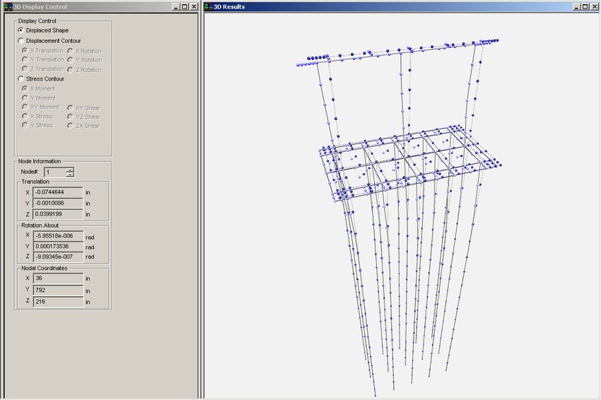
The deformed shape of the pier and bridge model can provide additional insight into the model
behavior. Click the (3D Results) button to view the deformed shape for the interior pier. The
deformed pier is shown in Figure 2.12. Nodal displacement data can be view by clicking on any node in
the pier model. The deformed shape for the entire bridge can be viewed by right-clicking the mouse in the
3D Results window and selecting “Bridge View” from the popup menu. This view is shown in Figure
2.13.
This concludes Example MP-2.
FB-MULTIPIER USERS MANUAL 1-39Figure 2.12 Pier Deformed Shape
Figure 2.13 Bridge Deformed Shape
FB-MULTIPIER USERS MANUAL 1-40MP-3. HIGHWAY BRIDGE IMPACT ANALYSIS
Shown in Figure 3.1 is a two-span highway overpass bridge, which was modeled in Example
MP-2. The bridge is supported by pile bent abutments and a general pier interior support. The bridge is
primarily subjected to vertical loads, but there is some concern about a possible vehicle collision force on
one of the columns in the pier. The bridge model developed in Example MP-2 will be modified to study
the effect of a time-dependent collision load on the pier column.
Dynamic
collision
force
60 ft
60 ft
Figure 3.1 Example MP-2, Two-Span Highway Overpass Structure
Select Open from the File menu and choose Example MP-2.in from the program directory (Figure 4.2).
FB-MULTIPIER USERS MANUAL 1-41Figure 3.2 Example MP-2, Bridge Model
In addition to a static analysis, FB-MultiPier offers dynamic analysis capabilities. The current
example considers only static loads. To switch to a dynamic analysis, select the Analysis data page and
choose “Dynamic” for the Analysis Type. Click “Yes” to remove all static load cases beyond load case 1
(a dynamic analysis can only contain a single load case). Notice that after selecting a dynamic analysis,
the “Dynamics” tree item becomes enabled. Select the Dynamics data page to specify the dynamic
parameters to use in the modeling and analysis. The Dynamics data page is shown in Figure 3.3.
FB-MULTIPIER USERS MANUAL 1-42Figure 3.3 Dynamics Data Page
The Dynamics data page contains a number of options for controlling the dynamic analysis.
Among these options are two types of dynamic analysis: 1) Time Step Integration and 2) Modal Response
Spectrum Analysis. This example will demonstrate the program capabilities for a time step integration
analysis. The Dynamics data page also contains options for including damping in the analysis using mass
and stiffness proportional damping factors as well as an option for modeling consistent or lumped mass
behavior. Three implicit time step iteration methods are also available and each requires parameters
indicating the time step and number of time steps to consider in the analysis. For this example, enter
“0.02” for the Time Step and “50” for the Number of Steps. The dynamic load function can be either
time-dependent loads or a ground acceleration record.
Click on the “Edit Functions” button to define a time-dependent load function. In the Edit Load
Functions dialog, select “Add Load Function” from the Load Function combo box. After doing so, “Load
Function 1” will be added to the combo box. To define the load function values, click on the “Edit
Function Values” button. Type “Vehicle Impact” for the name of the load function. Enter the 7 values
FB-MULTIPIER USERS MANUAL 1-43shown in Figure 3.4 and click “Ok”. The user-defined load function is shown in the plot in Figure 3.5.
Click “Ok” to close the plot dialog.
Figure 3.4 Load Function Values
Figure 3.5 Plotted Load Function
FB-MULTIPIER USERS MANUAL 1-44Now that the load function is defined, select the Load data page to apply the load to the model.
To apply the load to the interior pier, select “Pier #2” from the pier selection combo box in the toolbar.
This pier currently has a static load applied to it. This load will be replaced with the dynamic load
function. The letter “S” in front of Node 151 is used to indicate a static load. Click on the “S” to switch
the load to a dynamic load. Notice that the letter changes to a “D” to indicate a dynamic load and the
options on the page change as well. To apply the load in the transverse direction, enter “1” for the X
Direction factor. Also select the “Vehicle Impact” load function from the load function combo box. The
current state of the Load data page is shown in Figure 3.6. This completes the load definition and
application process. Note that both static and dynamic loads can be applied to a model, but not at the
same node. This example demonstrates dynamic load capabilities with the only static load being the self
weight of the bridge.
Figure 3.6 Load Data Page
This completes the modeling phase of this bridge model. To analyze the model under the applied
loads, click the (Analyze) button in the toolbar.
FB-MULTIPIER USERS MANUAL 1-45Results can be viewed after reaching a converged solution to the problem. Results are presented
per time step per pier and the pier selection combo box in the toolbar is used to switch between piers.
Click the (Pile Results) button to view the maximum results for the piles. The pile group for the
interior pier support is of particular interest since it must resist the collision force. Select “Pier #2” from
the pier selection combo box in the toolbar to view the results for the interior pier. FB-MultiPier allows
the user to view the maximum pile member force results and the corresponding time step (in a dynamic
analysis). To view the maximum pile shear force in the transverse direction, select “Shear2” from the
Member Force combo box as shown in Figure 3.7. Notice that the corresponding time step in which the
maximum Shear2 occurred is shown next to the pier selection combo box in the toolbar. In this example,
the maximum occurred in Time Step 16 (16 x 0.02 sec = 0.328 seconds into the analysis).
Figure 3.7 Maximum Pile Shear2 and Corresponding Time Step
To view the pier column results, click the (Pier Results) button. The outside pier column is of
particular interest since it must resist the collision force. FB-MultiPier allows the user to view the
FB-MULTIPIER USERS MANUAL 1-46maximum column and pier cap member force results and the corresponding time step (in a dynamic
analysis). To view the maximum column shear force in the transverse direction, select “Shear2” from the
Member Force combo box as shown in Figure 3.8. Notice that the corresponding time step in which the
maximum Shear2 occurred is shown next to the pier selection combo box in the toolbar. In this example,
the maximum occurred in Time Step 14 (14 x 0.02 sec = 0.28 seconds into the analysis).
Figure 3.8 Maximum Pier Column Shear2 and Corresponding Time Step
FB-MULTIPIER USERS MANUAL 1-47The maximum moment in the pier columns is also of interest for this example. To view the
maximum moment about the 3-axis, select “Moment3” from the Member Force combo box as shown in
Figure 3.9. Notice that the maximum moment also occurred in the same column at time step 14.
Figure 3.9 Maximum Pier Column Moment3 and Corresponding Time Step
To view the deformed shape of the pier, click the (3D Results) button. Next, click on Node
151 in the 3D model to view the displacement results at the impact point. After doing so, select the X
(transverse) translation option under “Results Plotting” and click the “Plot” button to view a displacement
time history. The resulting plot is shown in Figure 3.10. Other displacement directions can be plotted as
well. An animated movie of the time history response can be viewed by clicking the “Animate!” button.
Click the button again to stop the animation.
FB-MULTIPIER USERS MANUAL 1-48Figure 3.10 Displacement History at Impact Point
Before concluding this example it is important to note that the bearing reactions are also available
(in the output file) at every time step during the analysis. By viewing the bearing reactions at each pier,
the user can determine the amount of load that is shed to adjacent piers. Figure 3.11 shows the bearing
reactions at Time Step 14, where the shear force in the pier column reached a maximum value. Refer to
the FB-MultiPier Help Manual for the sign convention for the bearing reactions. The bearing reactions are
given an “L” or “R” designation, indicating the left or right row, respectively. The transverse bearing
reactions are located in the column labeled “FX.” Summing the reactions for Pier #1 (the first abutment)
indicates that only 19 kips of the dynamic impact (approximately is transferred to the first pier. Pier #3
also receives the same load from symmetry. In this example, the interior pier absorbs most of the impact.
FB-MULTIPIER USERS MANUAL 1-49BEARING REACTIONS
PIER #1
LOC L/R FX FY FZ MX MY MZ
(Kips) (Kips) (Kips) (Kip-ft) (Kip-ft) (Kip-ft)
--- --- ------ ------ ------ ------ ------ ------
1 R 9.1 24.1 -9.8 -97.6 120.7 -16.6
2 R -0.4 19.0 -87.9 -67.4 34.0 4.9
3 R 9.5 48.2 -158.8 -144.0 227.5 179.4
4 R 0.0 0.0 0.0 0.0 0.0 0.0
5 R 0.0 0.0 0.0 0.0 0.0 0.0
PIER #2
LOC L/R FX FY FZ MX MY MZ
(Kips) (Kips) (Kips) (Kip-ft) (Kip-ft) (Kip-ft)
--- --- ------ ------ ------ ------ ------ ------
1 L -28.1 10.0 -13.0 0.0 -166.0 10.5
2 L -10.6 -23.3 -49.2 0.0 -1.8 6.9
3 L -17.1 1.8 -64.1 0.0 -148.4 6.5
4 L 9.8 23.3 -63.3 0.0 3.2 -8.3
5 L 40.6 3.5 -42.8 0.0 84.7 -8.8
1 R -5.6 2.3 -59.8 -130.6 -141.6 9.0
2 R 11.5 23.6 57.4 -80.0 2.2 9.5
3 R -16.3 11.7 -106.6 -147.6 -157.2 -3.4
4 R -8.9 -23.2 72.0 -101.5 -3.1 -5.7
5 R 12.7 11.0 -90.0 -156.7 58.1 -9.5
PIER #3
LOC L/R FX FY FZ MX MY MZ
(Kips) (Kips) (Kips) (Kip-ft) (Kip-ft) (Kip-ft)
--- --- ------ ------ ------ ------ ------ ------
1 L 9.9 -7.7 3.1 52.1 99.2 -0.6
2 L -1.1 -10.2 -41.8 44.3 13.6 -3.6
3 L 0.4 -25.1 -50.9 66.8 78.4 -64.9
4 L 0.0 0.0 0.0 0.0 0.0 0.0
5 L 0.0 0.0 0.0 0.0 0.0 0.0
Figure 3.11 Bearing Reactions at Time Step 14
This concludes Example MP-3.
FB-MULTIPIER USERS MANUAL 1-50MP-4. HIGHWAY BRIDGE SEISMIC ANALYSIS
Shown in Figure 4.1 is a two-span typical highway overpass bridge, which was modeled in
Example MP-2. The bridge is supported by pile bent abutments and a general pier interior support. The
bridge is primarily subjected to vertical loads, but there is some concern about a possible seismic event.
The bridge model developed in Example MP-2 will be modified to study the effect of a time-dependent,
seismic loading (El Centro acceleration record).
Ground
acceleration
Ground
acceleration 60 ft
60 ft
Ground
acceleration
Figure 4.1 Example MP-2, Two-Span Highway Overpass Structure
Select Open from the File menu and choose Example MP-2.in from the program directory (Figure 4.2).
FB-MULTIPIER USERS MANUAL 1-51Figure
4.2 Example MP-2, Bridge Model
Example MP-2 utilized a concentrated load to simulate a vehicle collision event. This load is not
applicable in this example and should be removed. To do so, select “Pier #2” from the pier selection
combo box in the toolbar. Next, select the Load data page in the model data window and then click the
“Del” button to the right of the Node Applied list to remove the concentrated nodal load at Node 151. The
model is now ready for the seismic load application.
The current example considers only static loads. To switch to a dynamic analysis, select the
Analysis data page and choose “Dynamic” for the Analysis Type. Click “Yes” to remove all static load
cases beyond load case 1 (a dynamic analysis can only contain a single load case). In this example, the El
Centro ground acceleration record will be used to excite the bridge model. This record (provided with the
program) contains points at an equal time step of 0.02 seconds. In the Dynamics page, enter “0.02”
seconds for the time step, “1000” for the number of steps, and select “Ground Accel.” and click “Yes” to
FB-MULTIPIER USERS MANUAL 1-52proceed. Finally, enter “386.4” in/sec2 for the gravity factor for the acceleration record. These dynamic
parameters are shown in Figure 4.3.
Figure 4.3 Dynamics Data Page With Ground Acceleration Parameters
The next step is to provide a ground acceleration record for the seismic analysis. To do so, click
the “Edit Functions” button in the Dynamics data page. Next, click the “Read From File” button to load
an existing acceleration record. Click “Yes” to add a new (blank) dynamic load function. Select “1940 El
Centro.acc” from the program directory and click “Ok.” The selected load function is graphed in the load
function plot as shown in Figure 4.4. Note that load function values can be entered and modified using a
grid table by clicking the “Edit Function Values” button.
The final step in modeling the ground acceleration involves the application of the dynamic load
function. The currently defined ground acceleration must be applied in the Load data page for each pier.
Begin with the first pier (abutment) by selecting “Pier #1” from the pier selection combo box in the
toolbar. After selecting the Load data page, notice that a placeholder, labeled “Acc. (All Nodes),” is
provided for the ground acceleration. This placeholder indicates that the ground acceleration will be
applied to all nodes in the pier. Notice that the available load parameters change after selecting the
FB-MULTIPIER USERS MANUAL 1-53placeholder. To apply the ground acceleration in the transverse direction, enter “1” for the X Dir factor.
Leave all other direction factors as “0.” Finally, make sure the “1940 El Centro” record is selected to
apply to the pier. When done, confirm that the same acceleration record and direction have been applied
to the remaining piers by selecting “Pier #2” and “Pier #3” from the pier selection combo box.
Figure 4.4 El Centro Acceleration Record
Before analyzing the bridge model it is important to note that only 1000 time steps are being
considered even though the El Centro record contains 1576 points. This decision was made solely to
reduce the analysis time for this example. A complete analysis should consider the bridge behavior during
the entire seismic event.
This completes the modeling phase of this bridge model. To analyze the model under the applied
loads, click the (Analyze) button in the toolbar. The analysis will take several minutes depending on
the speed of the computer. Results can be viewed after reaching a converged solution to the problem.
Results are presented per time step per pier and the pier selection combo box in the toolbar is used to
switch between piers.
FB-MULTIPIER USERS MANUAL 1-54The amount of numerical results data is significant for a dynamic analysis. Keep in mind that
processing the data requires a significant amount of computer resources and the printed output file is
significantly larger than an output file from a static analysis. In fact, it is not uncommon to have more
than 100MB of results data for a dynamic analysis of a full bridge. Results data summaries are available
in order to assist the user in identifying maximum load conditions. For example, a summary of the
maximum internal forces in the piers (and the corresponding time step) is given at the end of the printed
output file. Additionally, the maximum internal force results and corresponding time step number can be
viewed using the graphical interface.
To view the maximum results for the piles, click the (Pile Results) button. To demonstrate
the plotting capabilities, select “Pier #2” from the pier selection combo box in the toolbar to view the
results for the interior pier. FB-MultiPier allows the user to view the maximum pile member force results
and the corresponding time step. To view the maximum pile shear force in the transverse direction, select
“Shear2” from the Member Force combo box as shown in Figure 4.5. Notice that the corresponding time
step in which the maximum Shear2 occurred is shown next to the pier selection combo box in the toolbar.
In this example, the maximum occurred in Pile #5 at Time Step 592 (592 x 0.02 sec = 11.84 seconds into
the analysis).
A displacement history for any node in the model can also be plotted, as shown in Figure 4.6.
Finally the displaced shape can be animated, using the “Animate!” button, to view the deformation
behavior over time. An animation control dialog is also available to play, pause, and quickly advance to a
particular time step during the animation. The “Animation Control” option is accessible from the toolbar.
This concludes the time history analysis portion of this example.
FB-MULTIPIER USERS MANUAL 1-55Figure 4.5 Maximum Pile Shear Force (Pile 5)
Figure 4.6 Displacement Response Record (Node 160 – Pier Cap End)
FB-MULTIPIER USERS MANUAL 1-56RESPONSE SPECTRUM ANALYSIS COMPARISON
FB-MultiPier provides a modal response spectrum analysis capability as an alternative to a time
step integration analysis. One key benefit of the response spectrum analysis is the rapid analysis time due
to the reliance on pre-computed maximum response quantities. A response spectrum analysis does have
several drawbacks, however. Most notably, the user must include enough modes in the analysis to capture
at least 90 percent of the structural response. The number of modes is generally obtained by trial and error
and can require several analysis attempts. Also, the modal analysis requires a linear material behavior in
order to correctly combine the modal contribution results. Despite these drawbacks, a comparison of both
dynamic analysis methods is presented here to provide some insight into the differences between the
methods.
The implementation of a response spectrum analysis in the FB-MultiPier program is somewhat
unique due to the fact that soils exhibit a nonlinear behavior under most types of loading. By definition,
modal analysis requires the linear combination of modal response quantities. FB-MultiPier, therefore,
provides an approximate response spectrum analysis by combining the modal response of a structure with
nonlinear properties (soil and possibly nonlinear pier and pile behavior). The modal analysis begins by
applying all static loads to the model, including self weight. The program then performs an eigen analysis
to generate the requested number of mode shapes and vibration frequencies while the model is in the
equilibrium (deformed) position. The response of each mode is then combined (CQC) using the direction
of excitation and the values for the response spectrum. Modal contribution factors are provided to indicate
the contribution of each mode. Final combined results are available for pier internal forces and
displacements. Note that the reported results only reflect the external loads applied to the structure
while in the equilibrium position. That is, the internal forces from static loads, such as self weight, are
not included in the results (because these loads were used to obtain the equilibrium position). Also, the
results are based off the initial soil stiffness. The soil stiffness is not adjusted using an iteration process.
Despite these factors, it is still possible to obtain results that are similar to those from a time step analysis.
FB-MULTIPIER USERS MANUAL 1-57You can also read