R Spatial and GIS Interoperability for Ethnic, Linguistic and Religious Diversity Analysis in Romania
←
→
Page content transcription
If your browser does not render page correctly, please read the page content below
R Spatial and GIS Interoperability
for Ethnic, Linguistic
and Religious Diversity Analysis
in Romania
Claudiu VINȚE (claudiu.vinte@ie.ase.ro)
The Bucharest University of Economic Studies

Titus Felix FURTUNĂ (titus@ase.ro)
The Bucharest University of Economic Studies

Marian DÂRDALĂ (dardala@ase.ro)
The Bucharest University of Economic Studies

                                     ABSTRACT
           Diversity aspects, particularly ethnic, linguistic and religious ones, have be-
come global, capturing a large interest in being extremely sensitive recently. Tradition-
ally, these had been issues concerning only particular countries and/or regions, due to
specific historical conditions. The recent waves of mass migration towards the wealth-
ier countries rose great problems regarding populations which come with radically dif-
ferent ethnic, linguistic and religious background compared to the local population. Our
research is focused on analysing ethnic, linguistic and religious diversity in Romania,
at Local Administrative Units level (LAU2), along with the segregation analysis regard-
ing the same aspects at county (NUTS3) and region levels (NUTS2) by integrating
R processing flexibility with and Geographic Information Systems (GIS) presentation
abilities. R programming language offers support for developing integrated analysis
solutions, based on specialized packages for computing diversity/segregation indices,
in connection with packages that allow processing and visualising data geospatially,
through interoperability with popular GIS, such as ArcGIS and QGIS. It is Romania
census data that is employed as data source for analysis, with a focus on the latest
census data from 2011.
           Keywords: R, GIS, Interoperability, Diversity Analysis, Segregation Analysis
           JEL classification: C610, C880

                             1. INTRODUCTION
        By their nature, administrative-territorial units are observations that
can be identified by geographical locations. R includes many functions for
reading, visualizing, and analyzing spatial data, as a base functions or as
functions belonging of others popular packages for spatial data processing.

Romanian Statistical Review nr. 4 / 2017                                               85
Such specialized packages are rgdal [1][2] for importing and exporting spatial
data, sp [3] and sf [16] for vector spatial data, raster for raster spatial data,
mapview for interactive visualization of maps. More in-depth details regarding
these packages are to be presented in the following chapter of this paper.
There are also specialized packages which provide interoperability between
R and Geographical Information Systems (GIS), such as arcgisbinding [15]
for ArcGIS, RQGIS for QGIS, RSAGA for SAGA GIS, or rgrass7 for GRASS
GIS. The ethnic, linguistic and religious diversity analysis is performed at two
levels, as following:
         1. at the counties level, in concordance with Nomenclature of
            Territorial Units for Statistics (NUTS3);
         2. at the communes, municipalities and cities level, according to Local
            Administrative Units (LAU2).

          2. PACKAGES, CLASSES AND METHODS
                 FOR SPATIAL DATA IN R
         The spatial data in R packages is currently broadly used. Many of
these packages employ specific data structures in order to create and handle
spatial data. The sp package introduces a coherent set of classes and methods
for the fundamental types of spatial data: points, lines, polygons etc. [2]. There
is entire suite of R packages which are dependent of sp package. Among the
main classes supplied by sp package for spatial data representation of points,
lines, polygons, and raster data types there are: SpatialPoints, SpatialLines,
SpatialPolygons, and SpatialPixels. All of these classes are extensions of
Spatial class, and they don’t contain non-spatial attributes. Furthermore,
these classes are extended by classes with additional non-spatial attributes,
containing the DataFrame suffix like SpatialPointsDataFrame, and which are
very much in line with the generic R data structures. In connection with the sp
package, there are other R packages like rgdal for reading/writing spatial data,
rgeos which provide the interface to the geometric processing system GEOS,
raster for raster level processing, maptools, ggmap, and tmap for spatial data
visualization.
         The newer package sf offers a synthetic and integrated solution for
processing spatial data in R, by cumulating the capabilities offered by sp,
rgdal, and rgeos packages. The main features offered by sf package are briefly
emphasized below.
         Geographic data I/O: Usually, the spatial data a stored in files or geo-
spatial data bases. The file format may be single raster abstract data model or
single vector abstract data model, according to Geospatial Data Abstraction
Library (GDAL) standards. This approach ensures the interoperability with

86                                  Romanian Statistical Review nr. 4 / 2017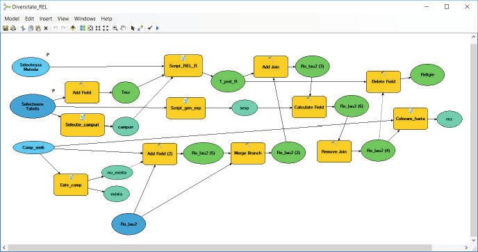
the formats employed by GIS like ArcGIS, GRASS GIS or QGIS. For reading
data in vector format sf package provides the function while writing vector
format data is achieved with sf::st_write() function. The objects returned by
sf::st_read() function are of data.frame type, which are readily available for
regular processing in R.
         Basic map making: The sf package offers the ability for easily
rendering maps by using plot() function. By default, sf creates a multi-panel
plot using all the non-spatial attributes of the data. The following code sample
draws the map of Romania, at the counties level (NUTS2), using plot()
function. The input data is read from a local “.shp” type file.

shpFile = choose.files(caption = “Romania shp file”,
filters = matrix(data = c(“Shp files”,”*.shp”)))
ro = sf::st_read(dsn = shpFile)
par(mar = c(0,0,1,0))
plot(x = ro[“cities”],main=”Romania’s map by no
of cities”)

         Ability to handle with geometric objects: The sf package offers the
ability to work with geometric object organized in collections. The handling
is achieved through sfc (simple feature collection) class. In order to combine
simple geometric objects is used st_sfc() function. Additionally, the created
geometric objected may have associated to them data regarding Coordinate
Reference System (CRS). The CRS data defines the manner in which the
spatial elements of the data relate to the Earth surface. Within sf package,
the object’s CRS related data can be fetched and set using the functions like:
st_crs () și st_set_crs ().
         Attribute data operations: The spatial data may contain a series of
non-spatial attributes associated to the geometric data type. Based on these
non-spatial attributes there can be conceived various ways to process vector
based spatial data, such as: sub-setting, aggregation or attribute data joining.
For this kind of processing there are available specialized packages like dplyr
[17], which offers an extended range of data handling capabilities at high
speed. These processing capabilities are facilitated by the flexibility offered
by data.frame class. Aceste prelucrari sunt facilitate de flexibilitatea oferita
de clasa data.frame.
         The following code sample shows data join and aggregation
employing the functions iner_join(), from din dplyr package, and aggregate()
from base, respectively. The iner_join() function connects a sf object to a data.
frame object creating as result a sf class object.

Romanian Statistical Review nr. 4 / 2017                                      87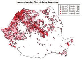
ro = sf::st_read(dsn = “maps\\RO_NUTS2\\Ro.shp”)
region = read.csv(file = “region.csv”)
ro_region = dplyr::inner_join(x = ro,y=region,by=”sj”)
sf::st_geometry(ro_region) = ro$geometry
par(mar = c(0,0,1,0))
ro_region_cities = aggregate(ro_region[“ORASE”], by =
list(ro_region$region), FUN = sum, na.rm = TRUE)
plot(x = ro_region_
cities[“ORASE”],main=”Romania’s map of regions
by number of cities”)
graphics::text(x =
sf::st_coordinates(sf::st_centroid(ro_region_cities)),
labels=ro_region_cities$Group.1)

         The geometric elements of the initial sf object are process by calling
the st_geometry() function. Essentially, the join type functions can be used
to enhance sf class objects with non-spatial attributed fetched from data.
frame class objects. The map resulted from the above sample includes as
well labels attached to the country’s regions, based on the level at which the
data aggregation has been conducted. The attribute which specify the region
had been previously added by calling inner_join(). The labels are shown in
the middle of polygons representing the regions. The functions st_centroid()
determines the centre coordinates for sf or sfc class objects.
         Spatial data operations: The standard functions for processing
spatial attributes of vector based data are sub-setting, joining and aggregation.
Sub-setting operations are achieved through specific spatial data functions
like intersect, touches, disjoint, crosses, contains etc. The following code
sample is used for determining the neighbours of a given county using st_
touches() function. This function returns the indexes of those elements of
which geometries have at least one point in common, but their interiors do not
intersect.

ro = sf::st_read(dsn = “maps\\RO_NUTS2\\Ro.shp”)
region = read.csv(file = “region.csv”)
bv = ro[ro$sj==”bv”,]
i = sf::st_touches(x = bv,y = ro)
par(mar = c(0,0,1,0))
plot(x = ro[i[[1]],1],main=”Neighbors of
Brasov (bv) County”, col=”red”)
graphics::text(x=sf::st_coordinates(sf::st_
centroid(ro[i[[1]],1])),
labels=ro$sj[i[[1]]])

88                                   Romanian Statistical Review nr. 4 / 2017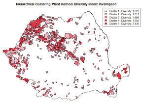
The spatial sub-setting operations can be achieved using the regular
R manner with square brackets. This way, the expression between the square
brackets is a spatial object. The sub-setting operation is in fact a join between
the object on which the sub-setting is being applied, and the object between
brackets. The following code sample shows the counties located in the centre
of Romania on a radius of 1 degree latitude and longitude. It uses CRS 4326,
based on Earth’s standard coordinate system (latitude/longitude).
ro = sf::st_read(dsn = “maps\\RO_NUTS2\\Ro.shp”)
 ro = sf::st_transform(x = ro,crs = 4326)
county = sf::st_union(x = ro[1,])
for(i in 2:nrow(ro)){
  county = sf::st_union(x=county, y = ro[i,])
}
center = sf::st_centroid(county)
mapCenter = sf::st_sf(geometry = center)
buff = sf::st_buffer(x = mapCenter, dist = 1.0)
par(mar = c(0,0,1,0))
plot(ro[buff,”ORASE”],main=”Counties from the
center by number of the cities”)
plot(x = buff,add=TRUE)

         In the case of spatial joins (executed on spatial data), the destination
objects receive the spatial attributes from the source objects, in the same manner
as in the case of simple joins (attribute join) simple attributes are added.
         In the case of spatial data aggregation, the grouping is executed
based on spatial attributes. The results consists in a number of items equals to
the aggregation entity’s number of items. For instance, in the previous code
sample, if we wanted to find out how many cities exists in the counties located
on a radius of 1 degree latitude and longitude we could write the following R
sequence:
> buff_agg = aggregate(x = ro[, “ORASE”], by = buff, FUN = sum)
> buff_agg$ORASE
[1] 64
         There would not make sense to attempt a spatial representation, since
there is no geographical entity identifiable by the ellipse of radiuses 1 degree
latitude and 1 degree longitude.
         The processing applied to raster based spatial data has a different
substratum, although they concern the same processing types. For instance, the
aggregation of vector based spatial data implies a dissolution of the polygons, while
in the case of raster based data the meaning is related to a change in resolution.
         The spatial aspects concerning the ethnic, linguistic and religious
diversity analysis do not require the usage of raster based type of spatial data;
hence we don’t treat this data type in this paper.

Romanian Statistical Review nr. 4 / 2017                                          89
3. STATISTICAL INSTRUMENTS IN GIS
In the current global context, GIS are more frequently employed to
add the spatial dimension to complex socio-economic phenomena analysis,
presenting the research outcome through digital geo-spatial maps. The
analysis is based either on dedicated statistical instruments for phenomena
spatial study, or on adaptive instruments used for studying the phenomena
at the territorial level. The former sets of instruments have been actually
developed within rigorously defined branches of Statistics (Spatial Statistics)
and Econometrics (Spatial Econometrics).
Most of the GIS based software have spatial analysis instruments
integrated within the software solution, or are capable to employ specialized
libraries provided with programming languages that have been adopted as
geo-processing languages, or there have been developed additional modules
for sustaining the interoperability with R statistical programming language.
Furthermore, there are software products dedicated to spatial analysis
like GeoDa, GeoDaSpace [12][13[14]. This software works with standard
formats for spatial data representation, along with the ability to handle no-
spatial data formats to allow for complex analysis and visualization of
processing results through maps containing adequate symbologies.
For example, an exhaustive treatment of the operations implemented
in Spatial Statistics Tools instrument from ArcToolbox component of ArcGIS,
with a special focus on Cluster analysis is provided by [11].
4. MEASUREMENT OF DIVERSITY
Many studies promote the species diversity indices as measures of
linguistic, ethnic or religious diversity. Such measure is linguistic diversity
index (LDI) [9][10]. Actually, this index is nothing but Shannon index [5],
used for diversity species measure, as we will be presenting in the following
paragraphs.
Thereby, the ethnic, linguistic and religious diversity analysis is
conducted using the following diversity indicators: species richness, and
measures of evenness.
Species richness represents the number of ethnic communities from a
certain territory. The simplest and most widely used index of species richness
is simply the number of groups or its logarithm.
The measure of evenness concerns the regularity of different groups’
distribution. The first regularity indicator that we considered is the dissimilarity
index of segregation [19], which is computed as follows:
90 Romanian Statistical Review nr. 4 / 2017n
1 ti ri
D=
2 ∑ T − R , where:
i =1
n is the number of spatial entities;
ti is the population of the target group in the spatial entity i;
T is the total population of the target group;
ri is the population of non-target groups in the spatial entity i;
R is the total population of the non-target groups.
The index ranges from 0.0 (complete integration) to 1.0 (complete
segregation).
Another measure of evenness is the Gini-Simpson [6][7] index. It is
n
computed as follows: S = 1 − ∑
pi2 where pi is the proportion of group i’s in
total population. i =1
A variation of this indicator is the inverse Simpson (or Rao):
1 .
Si = n
∑p
i =1
2
i
The third evenness measure that we took into account is entropy, in
the form Shannon-Weaver [5][7] index:
n
H = −∑ pi log b pi where b is the logarithm base.
i =1
Shannon-Weaver index is susceptible to relatively rare species, while
Simpson is susceptible to abundant species. Both Gini-Simpson and Shannon
indices varies between 0.0 and 1.0, with 1.0 indicating maximum diversity.
5. CASE STUDY UPON DIVERSITY ANALYSIS
Our diversity analysis is based on data supplied by the 2011 Romanian
census of people and housing [18]. The data is structured on ethnicity, mother
tongue, and religion. The territorial units that we refer to are: cities, counties,
regions, and macro-regions.
5.1 Computing diversity indices using R scripts within ArcGIS
ModelBuilder
In order to facilitate the geoprocessing workflow, and to increase
productivity when implementing complex operations, a visual programming
tool called ModelBuilder was developed as part of ArcGIS software [20][21].
ModelBuilder allows for constructing processing flows that may include R
Romanian Statistical Review nr. 4 / 2017 91and Python scripts as well. Figure 5.1.1 shows the processing flow built with
ModelBuilder for computing the diversity indices using vegan R package,
followed by maps plotting. R scripts integration within ArcGIS is ensured
by arcgisbinding package [22][21]. In the below diagram, the name of the R
script is Script_REL_R.
The processing flow for computing the diversity indices built with
ModelBuilder
Figure 5.1.1
We parameterized the R script such as to offer the ability to select
the desired diversity index (Shannon, Simpson or invSimpson), and the input
database table containing the census data regarding ethnicity, mother tongue,
or religion.
tool_exec=function(in_params,out_params)
{
library(RODBC);library(vegan);library(dplyr)
diversityTable=in_params[[1]]
diversityIndex=in_params[[2]]
columnsPar = in_params[[3]]
conn=odbcConnectAccess(“D:\\Diversitate\\Ro.mdb”)
key=”Cod”
dbTable=sqlQuery(conn, paste(“SELECT * FROM “,diversityTable,sep = “”))
columns = strsplit(x = columnsPar,split = “:”)
col1 = which(names(dbTable)%in%columns[[1]][1])
col2 = which(names(dbTable)%in%columns[[1]][2])
colKey=which(names(dbTable)%in%key)
tabDiv=select(tbl_df(dbTable),col1:col2)
tabSiruta=select(tbl_df(dbTable),colKey)
div=diversity(tabDiv,index=diversityIndex)
div = (div- min(div))/(max(div)-min(div))
92 Romanian Statistical Review nr. 4 / 2017div = round(x = div,digits = 3)
for(i in 1:length(div)){
updateCommand=paste(“UPDATE “,diversityTable,” SET Div=”,div[i],”
WHERE “,key,”=”,tabSiruta[i,1],sep=””)
sqlQuery(conn,updateCommand)
}
close(conn)
out_params[[1]] = in_params[[1]]
return (out_params)
}
Figure 5.1.2 illustrates the ethnic diversity in Romania, based on
values of ethnic diversity index.
ArcGIS generated map of Romania showing the ethnic diversity
Figure 5.1.2
5.2 Cluster analysis on diversity indices employing R Spatial
We constructed a synthetic representation of diversity by creating
partitions that include localities with diversity indices in near vicinity. The
approach achieved through clustering, the localities from a certain cluster are
represented geographically in a single shape. Therefore, the polygons afferent
to the localities belonging to a certain cluster are brought together under a
single shape, as a result of an aggregation operation based on the cluster
number (aggregate() function).
Figure 5.2.1 illustrates a hierarchical classification for ethnic diversity
structured in 5 clusters, based on values of Simpson diversity index.
Romanian Statistical Review nr. 4 / 2017 93There can be noticed the regions with a higher diversity are located in the
centre and north-west part of the country. On the other hand, Figure 5.2.2
shows the map of religious diversity. The classification is based on k-means
clustering.
Ethnic diversity Religious diversity
Figure 5.2.1 Figure 5.2.2
It is apparent that the religious diversity is greater, fact explained by the
traditional separation of ethnic communities in Moldavia and Transylvania in
Orthodox and Catholic or Greco-Catholic Christians. Moreover, the Hungarian
communities in Transylvania are Protestants, Catholics and Unitarians.
We found out that the ethnic and linguistic diversity in Romania
is almost exclusively explained through the contribution of Hungarian and
Romany population. Figure 5.2.3 illustrates the map of Romania’s ethnic and
linguistic diversity, respectively, without the contribution of Hungarian and
Romany population (linguistic diversity index - Shannon).
Ethnic and linguistic diversity in Romania, without Hungarian and
Romany population
Figure 5.2.3
94 Romanian Statistical Review nr. 4 / 2017The other 18 ethnic groups that we considered in our study generate a
very low diversity, isolated in a few number of localities. The fact that there are
insignificant differences between the ethnic diversity map and the linguistic
diversity map corroborates the conclusion that the vast majority of the ethnic
groups do use their native language.
5.3 Determining distribution regularity using R Spatial
Regarding the distribution regularity, it can be determined based on
the census data from the county level, following the distribution disparity
among cities within a given county. Figure 5.3 shows the Romany people
distribution within the country, at the county level. For each county, a pie
type graphic illustrates the weight of Romany population within the total
county’s population. The disparity index, (evenness) is significant where it
has an important weight relative to the territorial unit (county). The country
level, is appears the Romany population is fairly even distributed. There are
nevertheless differences when we go the county level. There are noticeably
higher values in the counties located in the eastern part of the country
(Moldavia). Regarding the religious disparity, we chose to emphasise the
disparity of Pentecostal population, due to the rapid expansion of this cult in
the recent years. There can be noticed higher values in eastern counties again,
but also in south-east and central counties. In these counties the cult members
are concentrated in some localities, missing from most parts of the county’s
territory.
Distribution of Romany and Pentecostal populations
Figure 5.3
Romanian Statistical Review nr. 4 / 2017 956. CONCLUSIONS AND FURTHER RESEARCH
In this paper we treat both aspects of integration and interoperability
that refer to integrating R scrips into GIS applications, and bringing R
processing sequences into GIS driven software solutions.
Our research is focused on analysing ethnic, linguistic and religious
diversity in Romania, at Local Administrative Units level (LAU2), along
with the segregation analysis regarding the same aspects at county (NUTS3)
and region levels (NUTS2) by integrating R processing flexibility with and
Geographic Information Systems (GIS) presentation abilities. R programming
language offers support for developing integrated analysis solutions, based
on specialized packages for computing diversity/segregation indices,
in connection with packages that allow processing and visualising data
geospatially, through interoperability with popular GIS, such as ArcGIS and
QGIS.
The spatial representation of data output proved to be crucial in
offering a synthetic perspective upon the ethnic, linguistic and religious
diversity, taken into account the granularity level at which the analysis was
conducted. In Romania there are 3181 localities, and table based analysis
could not possibly reveal the type of information that a geo-spatial approach
can offers. Due to article length considerations, the study does not include
all the maps the developed applications can generate, in order to support
exhaustive comparisons regarding ethnic, linguistic and religious diversity.
Nevertheless, there are findings of which relevance we want to emphasise:
• the fact that there are insignificant differences between the ethnic
diversity map and the linguistic diversity map corroborates the
conclusion that the vast majority of the ethnic groups have preserved
and do use their native language;
• the religious diversity the considerably greater due to confessional
no-uniformity of main ethnic groups: Romanians, Hungarians, and
Romany;
• the ethnic and linguistic diversity in Romania is almost exclusively
explained through the contribution of Hungarian and Romany
population; the other 18 ethnic groups that we considered in our
study generate a very low diversity, isolated in a few number of
localities.
We proved that GIS graphic representation capabilities can offer an
extremely useful spatial dimension to well establish data analysis technics
implemented in R, when it comes to data visualization. Our ongoing research
aims to design programming technics for integrating R processing with GIS to
interoperate at source code level.
96 Romanian Statistical Review nr. 4 / 2017References
1. Roger S. Bivand, Edzer J. Pebesma, Virgilio Gómez-Rubio, 2008, Applied Spatial
Data Analysis with R, Springer Science+Business Media, LLC,
2. Pebesma, Edzer, and Roger Bivand, 2017, Sp: Classes and Methods for Spatial
Data, https://CRAN.R-project.org/package=sp,
3. Bivand, Roger, Tim Keitt, and Barry Rowlingson, 2017, Rgdal: Bindings for the
Geospatial Data Abstraction Library. https://CRAN.R-project.org/package=rgdal
4. Patrick Sturgis, Ian Brunton-Smith, Jouni Kuha, Jonathan Jackson, 2014,
Ethnic diversity, segregation and the social cohesion of neighbourhoods in London,
Ethnic and Racial Studies, 2014, Vol. 37,No. 8, 1286–1309
5. Shannon, C. E. et Weaver, W., 1963, The Mathematical Theory of Communication,
University of Illinois Press
6. Simpson, E. H., 1949, Measurement of diversity. Nature 163(4148): 688
7. Eric Marcon, 2015, Mesures de la Biodiversite, Master, Kourou, France,
8. Whittaker, R. H., 1972, Evolution and Measurement of Species Diversity, Taxon,
21(2/3): 213-251
9. Joseph H. Greenberg, 1956, The Measurement of Linguistic Diversity, JSTOR, Vol.
32, No. 1, pp. 109-115
10. Steele, J, 2008, Population Structure and Diversity Indices, Genetics and Human
Prehistory, McDonald Institute for Archaeological Research. Chapter 18: 187-191
11. Reveiu, A., 2011, Techniques for Representation of Regional Clusters in
Geographical Information Systems, Informatica Economică vol. 15, no. 1/2011, Ed.
Inforec, Bucuresti, pp. 129–139.
12. https://spatial.uchicago.edu/software
13. http://gisgeography.com/qgis-arcgis-differences/
14. http://darribas.org/gds_scipy16/;
15. Marjean Pobuda, Using the R-ArcGIS Bridge: the arcgisbinding Package, https://
r-arcgis.github.io/assets/arcgisbinding-vignette.html
16. Edzer Pebesma, Roger Bivand, Ian Cook, Tim Keitt, Michael Sumner, Robin
Lovelace, Hadley Wickham, Jeroen Ooms, Etienne Racine, sf: Simple Features
for R, https://CRAN.R-project.org/package=sf
17. Hadley Wickham, Romain Francois, Lionel Henry, Kirill Müller, RStudio, 2017,
dplyr: A Grammar of Data Manipulation, https://CRAN.R-project.org/package=dplyr,
18. National Institute of Statistics, 2011, Population and Households Census 2011,
http://www.recensamantromania.ro/rezultate-2/
19. Rao, C. R., 1982, Diversity and dissimilarity coefficients: a unified approach,
Theoretical Population Biology 21(24-43)
20. Environmental Systems Research Institute, 2016, Inc., Executing tools in
ModelBuilder, http://desktop.arcgis.com/en/arcmap/10.3/analyze/executing-tools/
executing-tools-in-modelbuilder-tutorial.htm
21. Marian Dârdală, Titus Felix Furtună, Adriana Reveiu, Integrating R Scripts In
Gis, Vol. Education, Research & Business Technologies, Proceedings Of The
15th International Conference On Informatics In Economy (IE 2016), Cluj-Napoca,
Romania, June 02 –05, 2016, pp. 250-256
22. K. Krivoruchko, D. Pavlushko, 2015, Improving R and ArcGIS integration,
GRASPA 2015 Biennial Conference, Bari, 15-16 June, 2015
Romanian Statistical Review nr. 4 / 2017 97You can also read