Usage of GPUs in ALICE Online and Offline processing dur- ing LHC Run 3
←
→
Page content transcription
If your browser does not render page correctly, please read the page content below
arXiv:2106.03636v1 [physics.ins-det] 7 Jun 2021

                                                  Usage of GPUs in ALICE Online and Offline processing dur-
                                                  ing LHC Run 3

                                                  David Rohr1,∗ for the ALICE Collaboration
                                                  1
                                                      European Organization for Nuclear Research (CERN), Geneva, Switzerland

                                                                Abstract. ALICE will significantly increase its Pb–Pb data taking rate from
                                                                the 1 kHz of triggered readout in Run 2 to 50 kHz of continuous readout for
                                                                LHC Run 3. Updated tracking detectors are installed for Run 3 and a new two-
                                                                phase computing strategy is employed. In the first synchronous phase during
                                                                the data taking, the raw data is compressed for storage to an on-site disk buffer
                                                                and the required data for the detector calibration is collected. In the second
                                                                asynchronous phase the compressed raw data is reprocessed using the final cal-
                                                                ibration to produce the final reconstruction output. Traditional CPUs are unable
                                                                to cope with the huge data rate and processing demands of the synchronous
                                                                phase, therefore ALICE employs GPUs to speed up the processing. Since the
                                                                online computing farm performs a part of the asynchronous processing when
                                                                there is no beam in the LHC, ALICE plans to use the GPUs also for this second
                                                                phase. This paper gives an overview of the GPU processing in the synchronous
                                                                phase, the full system test to validate the reference GPU architecture, and the
                                                                prospects for the GPU usage in the asynchronous phase.

                                                  1 Introduction
                                                  ALICE (A Large Heave Ion Collider Experiment [1]) is undergoing a major upgrade dur-
                                                  ing the LHC long shutdown 2 in preparation for increasing its data taking rate during LHC
                                                  Run 3 [2]. This includes updates to the major tracking detectors ITS (Inner Tracking Sys-
                                                  tem [3]) and TPC (Time Projection Chamber [4]) as well as an upgrade to the computing
                                                  scheme within ALICE O2 (Online Offline [5]), comprising the three projects EPN (Event
                                                  Processing Nodes), FLP (First Level Processors), and PDP (Physics and Data Processing).
                                                  The readout will no longer be trigger-based but rather ALICE will record 50 kHz of minimum
                                                  bias Pb–Pb collisions in continuous readout. Instead of the classical approach with fast on-
                                                  line processing for triggers and QA (Quality Assurance) followed by the computing-intensive
                                                  offline event reconstruction, the processing happens in a synchronous and an asynchronous
                                                  phase. In Run 3 all recorded raw data are compressed and stored to an on-site disk buffer
                                                  during the synchronous phase. In parallel, the synchronous phase extracts all required data
                                                  for the detector calibration, followed by an intermediate step that produces the calibration ob-
                                                  jects. The asynchronous phase performs the full reconstruction of the data. It is split between
                                                  the compute nodes of the online computing farm and the GRID. Both synchronous and asyn-
                                                  chronous phases use the same software and the same infrastructure, but with different settings
                                                  and thresholds. The rationale behind using the online computing farm for the asynchronous
                                                       ∗ e-mail: drohr@cern.ch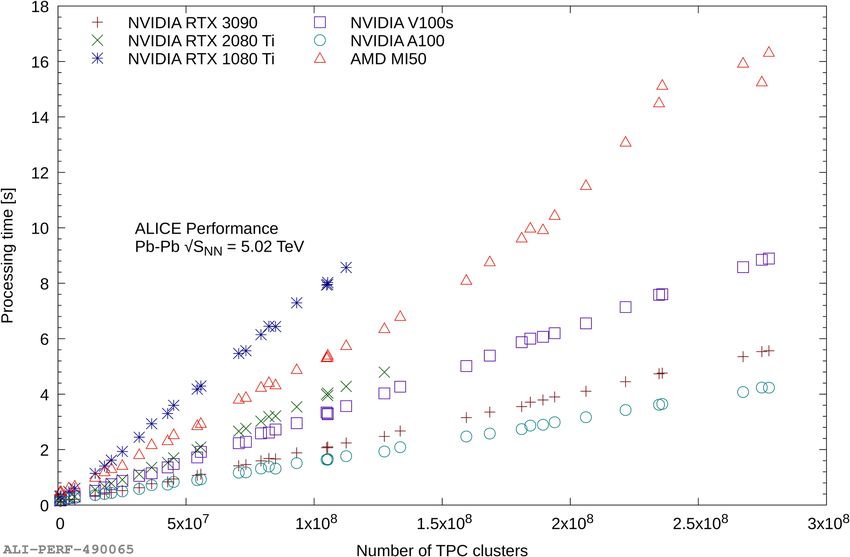
processing is that the LHC is without beam for a significant amount of time, and on top of
that the collision system is pp most of the time, which requires less computing resources than
Pb–Pb collisions. Hence, running only the synchronous processing, the online computing
farm would idle or operate at low load for most of the time.

2 ALICE Data Processing in Run 3
One general and significant change in the ALICE data processing in Run 3 is the switch
from the triggered readout to continuous readout. In the drift detectors like the TPC, there
are no single isolated events, but an overlap of multiple collisions, separated in time, which
translates almost linearly to the beamline coordinate. But since the time interval between
collisions is shorter than the TPC drift time, the tracks and the hits originating from the
individual collisions cannot be assigned to the vertices a priori. Instead, a larger bunch of
continuous data spanning multiple drift times is reconstructed together, and the assignment
of tracks to collisions happens only after the track reconstruction. The basic processing unit
for ALICE in Run 3 is thus not the event, but the Time Frame (TF), which contains by default
128 LHC orbits (around 10 ms) of continuous data. The processing scheme is illustrated in
Fig. 1.

                                              Data links from detectors          3.5 TB/s
                         FLP

                                                     Readout nodes
                                                                                  600 GB/s
                                                                                      data-taking

                                                  Synchronous processing
                         EPN Computing farm

                                                                                        During

                                               - Event / timeframe building
                                               - Calibration / Compression

                                                      Disk buffer
                                                                                      no beam
                                                                                       During

                                                Asynchronous processing
                                              - Reprocessing, full calibration
                                              - Full reconstruction
                                                                                       Compressed
                   Reconstructed Data                                                  Raw Data
                                                   Permanent storage                      < 100 GB/s

Figure 1. Illustration of the ALICE Run 3 processing scheme with two processing phases, synchronous
and asynchronous, and the storage to the disk buffer in between.

2.1 Synchronous Processing

The synchronous processing has two main objectives. First, the compression of the raw data
to Compressed Time Frames (CTF), which are stored to the disk buffer. And second, the
extraction of all data required for the calibration, such that the calibration tasks may run
afterwards without accessing the raw data again.
    The incoming raw data rate at 50 kHz Pb–Pb is over 3 TB/s, thus it is impossible to store
the data, even temporarily. Also a transfer over a longer distance would be complicated.
Instead, it must be compressed in real time to a manageable size in the on-site online
computing farm. The farm is split in two parts. The data enters the farm in the First Level
Processors (FLP) via the Common Readout Units (CRU) [6]. The CRUs are FPGA-based
PCI Express (PCIe) cards that receive the detector data via optical links, optionally perform
local processing in the user logic in the FPGA, and transfer the data to the memory of the
host. Each FLP sees only the data from the links connected to it, i. e. only parts of individual
detectors, but it has access to all data arriving from that link. From the FLPs the data is sent
over an Infiniband network to the Event Processing Nodes (EPN). The EPN is the larger
computing farm and provides the majority of the computing capacity. The event building
happens during this network transfer, which is arranged such that each EPN receives full
time frames, i. e. all data from all links for an individual time frame. Thus, the EPN sees the
data from all detectors, but only for the duration of one time frame. Calibration tasks can run
on both the FLPs and the EPNs. By design, tasks operating on link-level, which need access
to the continuous data stream of a link, i. e. more than one time frame, must run on the FLP.
Other tasks will generally run on the EPN, particularly those that need global information.
Data compression happens in both the FLPs and the EPNs. The detector with the by far
largest data volume is the TPC, contributing with more than 90% to the total data size. The
CRUs in the FLPs perform zero-suppression of the TPC data before shipping it to the EPNs,
reducing the rate from 3.5 TB/s to 600 GB/s. The EPNs further compress the data down to a
rate of around 100 GB/s, which is then stored to the disk buffer as CTFs. A common lossless
ANS [7] entropy encoding is employed as the last stage for all detectors, and individual
detectors may employ specialized prior compression steps.
The TPC compression is the most elaborate one, involving several steps [8], some of
which are not lossless. In particular, a clusterizing algorithms converts the raw ADC values
to hits, those are stored in custom data formats with only as many bits as necessary to
match the intrinsic TPC resolution. Hits of tracks not used for physics analysis are removed,
while the remaining hits are processed by entropy-reduction steps such as the track model
compression [8, 9]. By design the identification of the hits to be removed requires full
tracking in the TPC during the synchronous processing as prerequisite.
The most computing-intensive task of the calibration is the TPC space-charge distortion
(SCD) calibration [9, 10], which requires matching and refitting of ITS, TPC, TRD (Transi-
tion Radiation Detector), and TOF (Time of Flight) tracks. This requires track reconstruction
for several detectors, but with the increased Run 3 interaction rate, processing in the order
of one percent of the events is enough for the calibration. Consequently, the TPC tracking
for all collisions, as required for the data compression, is the dominant workload of the
synchronous processing.
2.2 Asynchronous processing
In contrast to the synchronous processing, the asynchronous processing includes the recon-
struction for all detectors, and for all events instead of only a subset. Therefore, the processing
workload for all other detectors except the TPC is much higher than during the synchronous
processing. For the TPC, in contrast, the clustering and the data compression is not necessary
during the asynchronous processing, while the tracking runs on a smaller input data set, as
a subset of the hits were removed during the data compression. Consequently, the TPC pro-
cessing needs less time in the asynchronous phase than in the synchronous phase. Overall,
the TPC contributes a significant part to the asynchronous processing, but it is not dominant.
In contrast to synchronous processing of raw data, which must happen exclusively on the
EPNs, the CTFs are available in the GRID. The asynchronous reconstruction will be split
between the EPN farm and the GRID sites. While the final distribution scheme is still to be
decided, currently it is assumed to split it to around one third for the online computing farm,
the Tier 0, and the Tier 1 sites each.2.3 The Event Processing Nodes (EPN) online computing farm
The EPN farm is tailored for the fastest possible TPC track reconstruction, which is the bulk
of the synchronous processing. GPUs have been shown to excel at this task in the ALICE
High Level Trigger (HLT) during Run 2 [11], hence the EPN farm provides the majority
of its computing power in the form of GPUs. The initial version of the O2 tracking was
derived from the HLT tracking, and it has been improved in many aspects since then [12].
These improvements include in particular a better track resolution matching the Run 2 offline
resolution, the treatment of data from continuous readout with overlapping collisions in the
TPC and the absence of absolute, a priori z-coordinates, SCD corrections, and efficiency
improvements to function with the five-fold increase of the TPC occupancy compared to
Run 2. Since the data cannot be buffered, the EPN computing capacity must be sufficient for
the highest data rates expected during Run 3, which is 50 kHz of Pb–Pb collisions. Thus, the
TPC processing speed together with the maximum TPC input data rate define the number of
GPUs in the farm. The rest of the farm is composed to ensure maximum GPU performance
and minimal cost for the server infrastructure. For instance the number of required servers
is a function of the number of GPUs and of how many GPUs fit in one server. Plugging
more GPUs in the same server reduces the number of servers enabling some cost-saving for
the overall farm. The reference configuration for the EPN computing farm are dual-socket
servers with 8 GPUs each.
During the synchronous phase, the GPUs will be fully loaded by the TPC reconstruction.
With an EPN farm providing 90 percent of its compute performance via GPUs, it is desirable
to maximize the GPU utilization also in the asynchronous phase. Since the relative contri-
bution of the TPC to the overall workload is much smaller in the asynchronous phase, GPU
idle times would be high and processing would be CPU-limited, if only the TPC part would
run on the GPU. Therefore, ALICE attempts to port more computing-intense reconstruction
steps onto the GPUs.
Still, the primary objective of the EPN farm, and also of the software effort, is to enable
synchronous data taking and processing at 50 kHz Pb–Pb rate. If the EPN farm is unable
to sustain the full rate, there is no fallback solution, and ALICE would inevitably lose data.
Therefore, the GPU software was developed with two scenarios in mind:
• Baseline scenario: This mandatory scenario contains the GPU processing steps re-
quired to ensure synchronous processing at 50 kHz Pb–Pb rate. In addition, processing
steps with either already existing or nearly final GPU versions (e. g. for ITS [13]),
which enables the GPU usage with little development effort, are included.
• Optimistic scenario: Here, the goal is to run as many components as possible on
the GPU. Obviously, processing steps with negligible computing workload should not
be ported, and porting individual short processing steps, which would require data
transfers forth and back, is avoided. Ideally, a chain of many consecutive computing
intense workloads should run on the GPU. The full track reconstruction for all detectors
in the central barrel is considered as a good candidate, but the GPU effort includes other
detectors as well.
Figure 2 shows the relevant processing steps of the central-barrel global-tracking chain, and
highlights which components belong to the synchronous or the asynchronous phase or to
both, whether they run only for a reduced subset of the collisions, whether they belong to
the baseline or the optimistic scenario, and the current state of the GPU development. All
GPU code is developed in a generic way that can target different GPU architectures and can
also run on the CPU [14]. Hence, all the components shown in Fig. 2 can run on the CPU as
well. It is important to note that there are working CPU-only versions of the components notGPU barrel tracking chain TPC Cluster
TPC3.1.2 PCI Express Bandwidth
The ALICE TPC code (which transfers the most data) is written with a pipeline such that
the transfer of input and output data overlaps with the processing [11]. As long as the PCIe
transfer is fast enough, the GPU will never idle. The average data rates sent over PCIe are
rather low, but it must be considered that there is a peak load during the TPC clusterization
phase, when all the TPC raw data must be shipped to GPU. In order to avoid stalling the GPU,
PCIe must keep step with this particular transfer. The required speed depends on the GPU
performance. The impact of different PCIe generations on the performance was measured
to be negligible, as long as the processing pipeline can fully hide the asynchronous PCIe
transfer behind the processing. For the MI50, even PCIe Gen 2 would be sufficient, showing
an overall performance decrease of around 1% vs. Gen 3 with no difference between Gen 3
and Gen 4. Some other GPUs require Gen 3 for the full performance.
3.1.3 Memory size
Two memory constraints must be considered. Since ALICE always processes a full time
frame at once, the full time frame must fit in GPU memory. Much effort is put into reusing
GPU memory for consecutive processing steps [15], but at all times the raw data and the
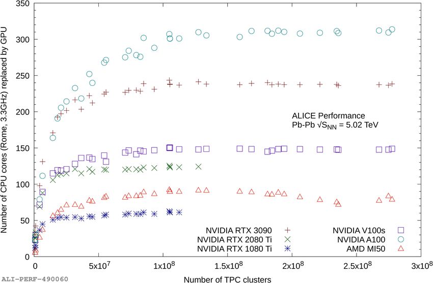
scratch data of one processing step must fit. Figure 3 shows the memory requirements. The
rightmost data points are for time frames with the default length of 128 LHC orbits and with
the occupancy of 50 kHz Pb–Pb. It is not planned to run with higher occupancies, but we
have verified that the TPC reconstruction performance behaves identically up to 256 LHC
orbits. Note that on top of the memory used by the application, the GPU runtime requires
additional memory, e. g., for the stack. It must also be considered that due to fluctuations in
centrality and luminosity, the number of TPC hits and thus the required memory size varies
to a small extent, demanding a certain margin. Taking this into account, a 24 GB GPU is
sufficient in the vast majority of cases and only less than 0.1% of the time frames would not
fit. Such time frames could easily be processed on the CPUs. The actual EPN farm will be
equipped with 32 GB GPUs, which do not have any memory limitation.
The potential reduction of the TF length was also studied.. At a length of 70 orbits, 16
GB GPUs would be sufficient. As is shown in the next section, the time frame length has no
general impact on the performance, as long as a certain minimum length of around 5 orbits
is exceeded. The processing time, for the most part, goes linearly with the input data size.
However, there can be certain non-linear effects for certain GPU models at certain sizes, such
as cache effects. This must be verified for a particular model and such sizes should be avoided.
Since time frames are processed individually, and at the end of each time frame there are
collisions with the TPC drift time reaching into the next time frame, there are a small number
of collisions that cannot be reconstructed [15]. There are technical solutions to recover these
collisions by storing a small amount of additional data, but in order to keep things simple and
to minimize the data loss, it was decided to stick to the 128 orbit time frame length.
Besides the GPU memory, there are also requirements on the host memory. With eight
GPUs, the host must hold at least 8 times the input data and buffers for the output data in
memory. In addition, to feed the GPU pipeline and to enable further pipelined processing of
the output on the CPU, an input queue containing four input time frames waiting in memory
and an output queue of eight time frames for postprocessing by CPU tasks are foreseen. With
around 5 GB input data size and around 10 GB output data size, this sums up to 220 GB
of memory. Adding memory for the CPU processing steps, network buffers, the operating
system, etc., it is clear that 256 GB of system memory will be insufficient, while 512 GB
should be enough (compare the measurements in section 3.3). It was not considered to usea non-power-of-two memory size, to equally load all 16 memory channels with identical
modules.
ALI-PERF-359004
Figure 3. Maximum GPU memory consumption Figure 4. Processing time of the synchronous re-
during synchronous reconstruction vs. input data construction on different GPUs vs. input data size.
size. Note that some GPUs are memory-limited.
3.2 Standalone benchmark
Performance is first evaluated by a standalone benchmark, which loads time frames in the
raw input format into memory, and processes them on the GPU in an endless loop as fast
as possible, without any additional framework code. The standalone test uses only a single
GPU, but it was tested to run eight GPUs in the same server independently in parallel, which
revealed an efficiency loss of less than 1%. Despite possible bottlenecks from PCIe transfers
or CPU processing, this should achieve 100% GPU load, while in reality around 99% GPU
load is achieved. Figure 4 shows the processing time of different GPU models against the
input data size measured in number of TPC hits. The speedup compared to a single CPU
core is shown in Fig. 5. It should be noted that these numbers are for the synchronous
reconstruction only, and are a bit biased towards the GPU since the employed clusterizing
algorithm performs much better on GPUs than on CPUs. For comparison, the speedup of
the MI50 GPU in the asynchronous reconstruction is in the order of 50 CPU cores. The
comparison was made to a single CPU core due to the vast majority of CPU models and core
counts. For comparing with multi-core processing on the CPU, one can practically scale
linearly with the number of cores. Figure 6 shows that on both AMD and Intel platforms the
scaling to multiple CPU cores is almost linear with an efficiency greater than 98% for 32 and
40 cores respectively. It also shows a significant improvement by enabling HyperThreading
/ SMT, which is thus active on the EPN farm.
From these numbers one can compute how many GPUs are required to cope with the
50 kHz Pb–Pb interaction rate, which is shown in Fig. 7 for different GPU models. Please
note that this estimate assumes continuous 100% GPU load, which is unrealistic in a real time
system. There will be inevitable latencies, and assuming 100% load, the farm could never
catch up any latencies that will appear. In addition, a margin is needed for two more reasons:
• There will be further improvements to the physics performance of the tracking, and un-
fortunately better performance does not imply faster code in this case. To the contrary,
if the track finding and cluster attachment efficiencies increase, the GPU has to fit more
tracks with more clusters, and the processing time will increase almost linearly.
• The upgraded TPC is a new detector that was never operated under 50 kHz Pb–Pb
conditions yet and thus not all parameters are exactly known.60
Speedup
ALICE Performance 05/27/2021
50
40
30
20 1 * Rome 32 Core 2.2 GHz
2 * Xeon 6230 20 Core 2.1 GHz
visual aid (slope=1)
10
0
0 10 20 30 40 50 60 70 80
ALI−PERF−490999 Number of threads
Figure 5. Speedup of different GPU models over a Figure 6. Speedup of multi-core processing on
single AMD Rome core running at 3.3 GHz vs. in- AMD and Intel CPUs. Thread placement is even
put data size (refer to Fig. 6 for the CPU multi- over CPU sockets and AMD CPU chiplets. Hy-
core performance). It is corrected for the CPU perThreaded / SMT cores are not used except for
load caused by the GPU processing, i. e. the av- the rightmost measurement points, which uses all
erage number of CPU cores used during the GPU cores. CPU frequencies were pinned to the indi-
processing is subtracted from the speedup. cated values.
Contrarily, there is also further possibility to speed up the code. Overall, a margin of
20% over the estimate of Fig. 7 is considered sufficient. In the case of the AMD MI50 model
of the actual EPN farm, this means around 2000 GPUs and thus 250 servers are required.
2500 75
70
ALICE Performance
Pb-Pb SNN = 5.02 TeV
2000 65
Number of GPUs needed for 50 kHz Pb-Pb
60
Temperature [°C]
1500
55
50
1000
45
40 GPU 1 GPU 6
500 GPU 2 GPU 7
35 GPU 3 GPU 8
NVIDIA RTX 3090 NVIDIA V100s GPU 4 CPU 1
NVIDIA RTX 2080 Ti NVIDIA A100 GPU 5 CPU 2
NVIDIA RTX 1080 Ti AMD MI50 30
0 0 50 100 150 200 250 300
0 5x10⁷ 1x10⁸ 1.5x10⁸ 2x10⁸ 2.5x10⁸ 3x10⁸
ALI-PERF-491405 Number of TPC clusters used for extrapolation Time [s]
Figure 7. Number of GPUs needed (computed Figure 8. GPU temperatures measured during
as processing time per time frame / time frame the full system test at 21°C environment tem-
length) for the synchronous reconstruction vs. in- perature. The strong fluctuations are due to the
put data size. Derived from the standalone bench- GPUs cooling down during the short idle peri-
mark for 50 kHz Pb–Pb rate for GPUs operating ods of 1 to 3 seconds in the full system test after
at steady 100% load. The measured processing around 10 seconds of full load for processing each
time obtained for a time frame (values of Fig. 4) time frame.
is scaled linearly by the number of the TPC hits
to the average number of hits in a time frame to
correct for centrality and luminosity fluctuations.
3.3 Full system test
In addition to the standalone benchmarks, a full system test of an EPN server prototype
was conducted in preparation of the EPN Production Readiness Review (PRR). The test
was conducted on a prototype server with two 64 core Rome CPUs, out of which two times32 cores were disabled in the BIOS to match the reference configuration. The server is
equipped with 512 GB of RAM, one Infiniband HCA, and eight AMD MI50 GPUs. Due
to GPU availability at that time, the 16 GB model was used, which limited the time frame
length to 70 orbits for the test. For validation, the same test was also successfully performed
on a server with two NVIDIA 2080 Ti GPUs. The full system test is limited to a single
server. However, since all servers are identical and are processing individual time frames
independently, there is no difference compared to testing multiple servers, except that it
takes more time to obtain an acceptable statistical precision. Since no setup with enough
FLP servers providing the input was available, time frames were replayed from within the
EPN memory without event building. The CPU overhead for the network transfer and event
building was measured independently to be six CPU cores or less. This number is added to
the CPU load measurements of the full system test.
The biggest difference to the standalone benchmark is that the GPUs are not processing
time frames as fast as possible, but time frames are published at a fixed rate and are then
processed by the full synchronous tracking chain including the CPU components (see Fig. 2).
It should be noted that some CPU components for some detectors were not ready at the time
of the test. Conservatively estimated, the included components account for at least 80% of the
total CPU processing workload, thus 25% is added on top of the CPU processing workload
measured in the full system test. The distribution scheme at a fixed rate means that the GPUs
will not be loaded at 100%, but close to it if the rate is chosen aggressively. The results
1
shown below are for a rate that corresponds to 250 of the 50 kHz Pb–Pb rate, which will reach
1
each single server out of the 250 server farm. The tests were repeated with 230 of the rate
to demonstrate a sufficient margin, which worked without any problems while CPU load and
buffer usage increased accordingly.
Figure 8 shows the GPU temperatures measured throughout the tests, which never ex-
ceeded 75◦ C, leaving 15◦ headroom to the 90◦ C temperature at which the GPUs begin to
throttle.
Figure 9 shows the CPU usage during the full system test measured as number of cores
used. The maximum CPU load was 44 cores. Out of these, 25 cores were used for the CPU
processing steps, which must be inflated by 25%. Adding six cores for network transfers and
event building on top, the full system test demonstrates that 56 cores are sufficient for the
synchronous processing. The EPN farm employs two 32 core processors, having a margin of
eight cores, and all SMT cores on top.
Figure 10 shows the memory usage during the full system test. The memory is split in
four regions. There are two Shared Memory (SHM) regions, one per NUMA (Non Uniform
Memory Architecture) domain, which are used for the data exchange between the various
processing components. Basically the EPN operates as two virtual EPNs with four GPUs
each, one per NUMA domain, however with a common input by the one Infiniband network
adapter. A third shared memory region in interleaved memory is used for the input. The
remaining non-SHM memory of the host is available as scratch memory for the processes.
Currently, one disadvantage of this approach is that free memory cannot be moved at runtime
between the regions. Thus each region must maintain a margin of free memory. The total free
memory of the server is the sum over the four regions, but if one region runs out of memory,
the processing will stall and create back pressure, until some memory is freed.
The natural way to verify that the server can cope with a certain rate is to observe the
memory buffers. If the fixed rate exceeds the processing capacity, the published input data
will start fill up the input buffers and the remaining buffer size will go to zero causing back
pressure. If the memory usage is constant over time, the processing speed is sufficient. This
1
is the case for an EPN server processing 230 of the 50 kHz Pb–Pb rate.45
SHM Input Segment
140 Non SHM memory
40 SHM Segment NUMA Domain 0
SHM Segment NUMA Domain 1
120
35
100
Free memory [GB]
CPU load [cores]
30
80
25
60
20
15 40
10 20
5 0
0 50 100 150 200 250 300 0 50 100 150 200 250
Time [s] Time [s]
Figure 9. Number of CPU cores used during the Figure 10. Memory usage during the first 5 min-
first 5 minutes of a full system test with eight utes of a full system test with 8 GPUs at 50 kHz
1
GPUs at 250 of the 50 kHz Pb–Pb data rate. The Pb–Pb rate. The free memory in the four distinct
load is smaller during the startup and then oscil- memory regions is shown. After around 90 sec-
lates around 38 cores due to small fluctuations of onds into the test, the memory utilization is fully
the load of the CPU parts of the reconstruction. stable.
4 Conclusions
The ALICE data processing scheme for Run 3 was described and the results of the full system
test conducted for the synchronous event reconstruction presented. The baseline solution
for using GPUs in the computing-intense workloads of the synchronous processing is fully
implemented and established. The 250 servers of the reference configuration, each equipped
with eight AMD MI50 GPUs, two 32-core Rome CPUs, and 512 GB of memory, are capable
of handling the Pb–Pb interaction rate of 50 kHz with roughly 20% margin. One GPU of
the employed model replaces around 50 CPU cores. On top of that, ALICE is aiming for a
more optimistic scenario to port the full central-barrel tracking chain to the GPU. This effort
is ongoing, but already several components beyond the synchronous reconstruction baseline
are available on the GPU. In parallel, other subdetectors not taking part in the central-barrel
tracking are investigating GPU adoption independently. All GPU code is written in a generic
way, such that GPU platforms can be switched easily, and the same algorithms run also on
the CPU.
References
[1] ALICE Collaboration, “The ALICE experiment at the CERN LHC”, J. Inst. 3 S08002
(2008)
[2] ALICE Collaboration, “Upgrade of the ALICE Experiment: Letter of Intent”, CERN-
LHCC-2012-012 (2012)
[3] ALICE Collaboration, ‘Technical Design Report for the Upgrade of the ALICE Inner
Tracking System“, CERN-LHCC-2013-024 (2013)
[4] ALICE Collaboration, “Technical Design Report for the Upgrade of the ALICE Time
Projection Chamber”, CERN-LHCC-2013-020 (2013)
[5] ALICE Collaboration, “Technical Design Report for the Upgrade of the Online-Offline
Computing System”, CERN-LHCC-2015-006, ALICE-TDR-019 (2015)
[6] O. Bourrion et al., “Versatile firmware for the Common Readout Unit (CRU) of the LHC
ALICE experiment”, Proceedings of TWEPP19, arXiv:1910.08804
[7] M. Lettrich, “Fast Entropy Coding for ALICE Run 3”, PoS(ICHEP2020)913[8] D. Rohr for the ALICE Collaboration, “Global Track Reconstruction and Data Com- pression Strategy in ALICE for LHC Run 3”, Proceedings of CTD2019 (2019) arXiv:1910.12214 [9] D. Rohr for the ALICE Collaboration, “Tracking performance in high multiplicities en- vironment at ALICE”, Proceedings of 5th Large Hadron Collider Physics Conference (2017), arXiv:1709.00618 [10] D. Rohr for the ALICE Collaboration, “Overview of online and offline reconstruction in ALICE for LHC Run 3”, Proceedings of CTD 2020 (2020) arXiv:2009.07515 [11] ALICE Collaboration, Real-time data processing in the ALICE High Level Trigger at the LHC, CPC 242 25 (2019), arXiv:1812.08036 [12] D. Rohr for the ALICE Collaboration, “Track Reconstruction in the ALICE TPC using GPUs for LHC Run 3”, Proceedings of CTD2018 (2018) arXiv:1811.11481 [13] M. Puccio for the ALICE Collaboration, “Tracking in high-multiplicity events”, Pro- ceedings of Science 287 043 (2017) doi:10.22323/1.287.0043 [14] D. Rohr, V. Lindenstruth, “Portable and Vendor-Independent Low-Level Programming and Performance Benchmarking for Graphics Cards and Processors”, Proceedings of 2017 IEEE 19th HPCCWS (2017) [15] D. Rohr for the ALICE Collaboration, “GPU-based reconstruction and data compres- sion at ALICE during LHC Run 3”, Proceedings of CHEP 2019 (2019) arXiv:2006.04158
You can also read