Time Series Classification of Cryptocurrency Price Trend Based on a Recurrent LSTM Neural Network - JIPS
←
→
Page content transcription
If your browser does not render page correctly, please read the page content below
J Inf Process Syst, Vol.15, No.3, pp.694~706, June 2019                                                                                          ISSN 1976-913X (Print)
https://doi.org/10.3745/JIPS.03.0120                                                                                                             ISSN 2092-805X (Electronic)

   Time Series Classification of Cryptocurrency Price Trend
        Based on a Recurrent LSTM Neural Network
           Do-Hyung Kwon*, Ju-Bong Kim**, Ju-Sung Heo*, Chan-Myung Kim***, and Youn-Hee Han**

Abstract
In this study, we applied the long short-term memory (LSTM) model to classify the cryptocurrency price time
series. We collected historic cryptocurrency price time series data and preprocessed them in order to make
them clean for use as train and target data. After such preprocessing, the price time series data were
systematically encoded into the three-dimensional price tensor representing the past price changes of
cryptocurrencies. We also presented our LSTM model structure as well as how to use such price tensor as input
data of the LSTM model. In particular, a grid search-based k-fold cross-validation technique was applied to find
the most suitable LSTM model parameters. Lastly, through the comparison of the f1-score values, our study
showed that the LSTM model outperforms the gradient boosting model, a general machine learning model
known to have relatively good prediction performance, for the time series classification of the cryptocurrency
price trend. With the LSTM model, we got a performance improvement of about 7% compared to using the GB
model.

Keywords
Classification, Gradient Boosting, Long Short-Term Memory, Time Series Analysis

1. Introduction
  In the stock market, it is common to generate profit by using algorithm trading instead of direct human
investment. Grove et al. [1] investigated 136 cases and concluded that mathematical models yield better
results than humans. Actually, various attempts and studies have been scientifically conducted with
regard to stock price prediction [2].
  Numerous cryptocurrencies have been developed recently based on blockchain [3,4], and a
cryptocurrency market has been formed. Especially, bitcoin is attractive in a variety of fields such as
economics, cryptography, and computer science due to the unique nature of the combination of
encryption technology and currency units [5,6]. A cryptocurrency market has a relatively short history
compared to the stock market. Fundamentally, both stock and cryptocurrency price data have arbitrary
characteristics as time series data, but the latter has higher volatility, and their prices fluctuate heavily.
  A cryptocurrency market is different from the existing stock market, and it has relatively many new

※ This is an Open Access article distributed under the terms of the Creative Commons Attribution Non-Commercial License (http://creativecommons.org/licenses/by-nc/3.0/) which
permits unrestricted non-commercial use, distribution, and reproduction in any medium, provided the original work is properly cited.
Manuscript received April 17, 2019; first revision May 17, 2019; accepted May 30, 2019.
Corresponding Author: Youn-Hee Han (yhhan@koreatech.ac.kr)
* Interdisciplinary Program in Creative Engineering, Korea University of Technology and Education, Cheonan, Korea ({dohk, chil1207}
    @koreatech.ac.kr)
** Dept. of Computer Engineering, Korea University of Technology and Education, Cheonan, Korea ({rlawnqhd, yhhan}@koreatech.ac.kr)
*** Advanced Technology Research Center, Korea University of Technology and Education, Cheonan, Korea (cmdr@koreatech.ac.kr)

www.kips.or.kr                                                                                                                                        Copyright© 2019 KIPS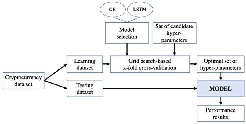
Do-Hyung Kwon, Ju-Bong Kim, Ju-Sung Heo, Chan-Myung Kim, and Youn-Hee Han

features [7]. Thus, in addition to the existing stock market prediction techniques, it is necessary to apply
new prediction techniques suitable for the cryptocurrency market. Although many related studies have
been conducted in the field of stock price, there are few studies on cryptocurrency price prediction.
  The purpose of this paper is to use a deep learning model [8] to predict the price trend of
cryptocurrencies without manual work. In detail, we aimed to construct our long short-term memory
(LSTM) model to classify the price time series direction (price-up or price-down) for an individual
cryptocurrency after a predefined time based on the past price time series changes of cryptocurrencies.
In particular, we tried to explore how to construct the training and target data from cryptocurrency price
time series data, so that they are suitable for input for the proposed LSTM model. We also demonstrated
the LSTM model’s superiority in prediction performance by comparing the f1-score values with those of
the gradient boosting model, a general machine learning model known to have relatively good prediction
performance.
  The rest of this paper is organized as follows: Section 2 briefly reviews some existing literature related
to cryptocurrency price prediction; Section 3 discusses how to collect and preprocess the cryptocurrency
price time series data and how to construct the train and target data for the LSTM model; Section 4
describes the proposed LSTM model and presents techniques for finding optimal model parameters;
Section 5 outlines the evaluation results of the LSTM model’s prediction performance; Finally, Section 6
presents the conclusion.

2. Literature Review
   A cryptocurrency market has many new features not found in the existing traditional stock market.
Traditional stock exchanges have their own trading sessions (e.g., from 09:00 am to 15:30 pm) with no
trading during state holidays or even weekends in most cases. In contrast, cryptocurrency exchanges are
available 24/7, and they instantly react to any event. Thus, if one is fast enough, one can make profits via
prompt transactions. Note, however, that it also means that traders should be online almost all the time
lest they miss out on opportunities. On the other hand, cryptocurrencies are highly volatile compared to
the traditional stock market. The cryptocurrency market is also easily manipulated unlike the stock
market, so the cryptocurrency price could easily increase or decrease. Lastly, cryptocurrency trading
requires the investors to store the coins themselves, and these assets are really vulnerable because new
traders are unsure as to how to secure their storage. These features make the prediction of the
cryptocurrency price difficult, and there is growing demand for new analytical techniques suitable for the
cryptocurrency market.
   Jang and Lee [7] proposed a Bayesian neural network model to predict the bitcoin price based on the
blockchain information involved in bitcoin's supply and demand and verified that the latest bitcoin price
has good predictive performance. Nonetheless, their model is limited to Bitcoin since the blockchain
information is not easy to obtain for other cryptocurrencies.
   Kim et al. [9] analyzed user comments in online social media to predict the price and number of
transactions of cryptocurrencies and showed that the proposed one-dependence estimator (AODE)
method is applicable to cryptocurrency trading by simulated investment. Note, however, that the method
depends only on social media and does not use any past price data, which are the most credible ones for
predicting the future price of cryptocurrencies.

                                                        J Inf Process Syst, Vol.15, No.3, pp.694~706, June 2019 | 695
Time Series Classification of Cryptocurrency Price Trend Based on a Recurrent LSTM Neural Network

  To address the portfolio management problem, Jiang et al. [10] proposed a deep reinforcement learning
method that directly produces the portfolio vector with historic cryptocurrency price data gathered from
Poloniex API as input. A back-test experiment was carried out on a cryptocurrency market, and the
performance was compared with 3 benchmarks and 3 other portfolio management algorithms, garnering
positive results. Nevertheless, their study is hardly an individual cryptocurrency trend prediction since
they proposed a portfolio management approach that determines which cryptocurrency requires heavy
investment.
  Radityo et al. [11] studied several multi-layer perceptron-based neural network models to predict the
price of Bitcoin. Their study opens new possibilities for future deep learning research on the
cryptocurrency price trend. Heo et al. [12] collected and processed several cryptocurrency price data
through Bithumb API. They then used the gradient boosting (GB) model, which is a representative data-
driven learning-based machine learning model, and let the model learn the price data change of
cryptocurrency. They also found the most optimal model parameters in the verification step and finally
evaluated the prediction performance of the cryptocurrency price trends. Their study showed that the GB
model’s f1-score is at most around 0.63, which is not a high prediction performance. Note, however, that
they did not use a deep learning model for the prediction and presented no comparison results between
the GB model and a deep learning model.

3. Data Processing
  This section describes the process of collecting cryptocurrency price data and reconstructing them for
use as training data. The data is collected by Bithumb API (https://www.bithumb.com/u1/US127). They
are initially mixed with various abnormal data, so they need to be preprocessed.

3.1 Data Collection and Preprocessing
  We collected cryptocurrency price values every 10 minutes. The collected data has five features: open
price, close price, high price, low price, and volume at each time epoch (i.e., every 10 minutes). We
considered seven kinds of cryptocurrency to be used in this work: BTC (Bitcoin), ETH (Ethereum), XRP
(Ripple), BCH (Bitcoin Cash), LTC (Litecoin), DASH (Dash), and ETC (Ethereum Classic), including
one fiat currency, KRW (Korean Won). The price and volume data were collected from 0:00 on June 9,
2017 to 09:00 on May 8, 2018 through Bithumb API.

Table 1. Example of the collected raw BTC price data
  Index              Time epoch                   Open price         Close price        High price   Low price   Volume
    1             2017-06-02 08:50:00              3121000            3130000            3142000      3121000     99.295
    2             2017-06-02 09:00:00              3130000            3142000            3143000      3130000    105.998
    3             2017-06-02 09:09:00              3142000            3141000            3147000      3132000    101.861
    4             2017-06-02 09:10:00              3142000            3143000            3146000      3141000     88.417
     5            2017-06-02 09:20:00                 -                   -                 -            -           -
    6                  Missing                     Missing            Missing            Missing      Missing    Missing
    7                  Missing                     Missing            Missing            Missing      Missing    Missing
    8             2017-06-02 09:50:00              3100000            3200000            3222000      3190000    182.123
    9             2017-06-02 09:59:00              3200000            3100000            3112000      3088000     98.762
    10            2017-06-02 10:10:00              3100000            3099000            3110000      3087000    177.615

696 | J Inf Process Syst, Vol.15, No.3, pp.694~706, June 2019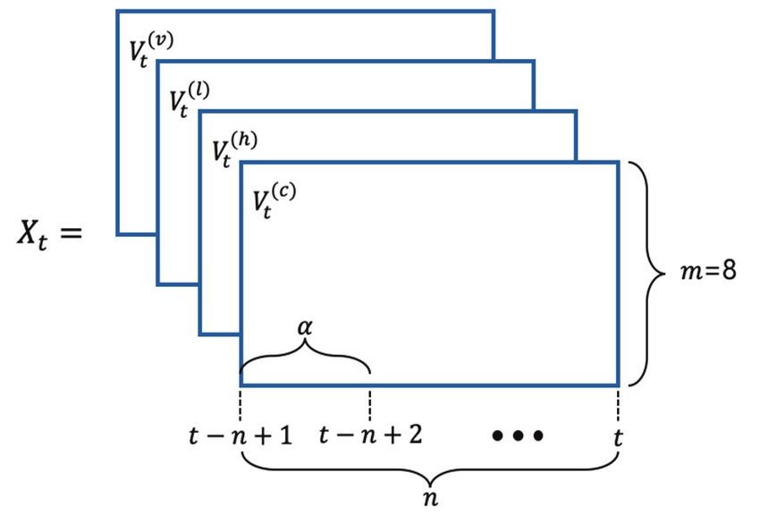
Do-Hyung Kwon, Ju-Bong Kim, Ju-Sung Heo, Chan-Myung Kim, and Youn-Hee Han

  Table 1 shows an example of the collected raw BTC price data. The collected data includes (1) normal
data (Indices 1, 2, 4, 8, and 10 in Table 1), (2) missing data, (3) empty data, and (4) non-matching data.
Missing data means data that has not been collected at a time interval of 10 minutes (Indices 6 and 7 in
Table 1). Empty data refers to data collected at a time interval of 10 minutes but is empty (Index 5 in
Table 1). Non-matching data is data that does not fit perfectly every 10 minutes (Indices 3 and 9 in Table
1)—the time information of the non-matching data is underlined. If certain data is empty or missed, then
the values of the previous normal data are copied to fill the value of the abnormal data. For example, in
the case of missing data, the previous data are copied, and the time information is properly inserted; the
case of empty data is also processed in the same manner. For non-matching data, if there are already
normal data collected at 10-minute intervals, the non-matching data whose time is closest to the normal
data is removed (Index 3 in Table 1). Otherwise, the time information of the data is updated with the time
adjusted to correct 10-minute intervals (Index 9 in Table 1). Table 2 shows the preprocessed data. It has
one less record than the raw data of Table 1, since the record whose index is 3 in Table 1 is removed.

Table 2. Preprocessed BTC price data for the raw data of Table 1
  Index          Time epoch            Open price       Close price            High price    Low price         Volume
    1         2017-06-02 08:50:00       3121000          3130000                3142000       3121000           99.295
    2         2017-06-02 09:00:00       3130000          3142000                3143000       3130000          105.998
    3         2017-06-02 09:10:00       3142000          3143000                3146000       3141000           88.417
    4         2017-06-02 09:20:00       3142000          3143000                3146000       3141000           88.417
    5         2017-06-02 09:30:00       3142000          3143000                3146000       3141000           88.417
    6         2017-06-02 09:40:00       3142000          3143000                3146000       3141000           88.417
    7         2017-06-02 09:50:00       3100000          3200000                3222000       3190000          182.123
    8         2017-06-02 10:00:00       3200000          3100000                3112000       3088000           98.762
    9         2017-06-02 10:10:00       3100000          3099000                3110000       3087000          177.615

3.2 Training and Testing Data
  Our training and testing data are encoded to the three-dimensional price tensor using the preprocessed
data. The price tensor is defined as similar to the one introduced in [10]. Price tensor at epoch
                                                  ( )       ( )     ()          ( )
consists of four two-dimensional matrices           ,     ,     , and     , which represent close price, high
price, low price, and transaction volume, respectively, for every unit of time . Open price is not included
in a price tensor because it usually equals the close price of the previous time epoch. In our study, the unit
of time will be 10, 30, or 60 minutes.
                                                                                      ( )                       ( )
  The close price for epoch of the -th cryptocurrency is denoted by                   , . On the other hand,    ,     is the
                   ()                                       ( )
high price data,   ,    is the low price data, and           ,    is the transaction volume of epoch . The 0-th
cryptocurrency represents KRW (Korean Won), and its tensor value is always 1 regardless of epoch ,
since we assume that it plays the role of standard currency.

                                        ( )       ()          ( )        ( )
                                         ,    =    ,    =      ,    =     ,    =1                                        (1)

  The price tensor at a time epoch includes the past price and volume data for the unit of time . We
call the window size. If = 30 and = 50, price tensor includes the price data during 30 × 50 =
1500 minutes. Let be the number of cryptocurrencies including the base currency, and it is set to 8

                                                              J Inf Process Syst, Vol.15, No.3, pp.694~706, June 2019 | 697
Time Series Classification of Cryptocurrency Price Trend Based on a Recurrent LSTM Neural Network

(KRW, BTC, ETH, XRP, BCH, LTC, DASH, ETC) in this study. Fig. 1 shows the data structure of the
price tensor at time epoch for window size , the unit of time , and the eight cryptocurrencies
                                                                                                                               ( )        ( )
(i. e. ,   =8). When operator ⊘ is defined as element-wise vector division, the four matrices                                        ,          ,
  ()           ( )
       , and         for epoch and 0                   7 are as follows:

                                ( )         ( )             ( ) ( )             ( )    ( )                ( )
                                      =      ,         ⊘    , | ,         ⊘      , |⋯| ,            ⊘      , |

                               ( )          ( )             ( ) ( )             ( )    ( )                ( )
                                      =      ,         ⊘    , | ,         ⊘      , |⋯| ,            ⊘      , |

                                ()          ()              ( ) ()              ( )    ()                 ( )
                                      =     ,          ⊘    , | ,        ⊘       , |⋯| ,            ⊘      , |

                               ( )          ( )             ( ) ( )             ( )   ( )                 ( )
                                      =      ,         ⊘     , | ,        ⊘     , |⋯| ,             ⊘     , |                             (2)

  Eq. (2) shows that all the values are divided by the corresponding last price or last volume, so they are
well-normalized.

Fig. 1. Data structure of price tensor at the time epoch ( : the window size, : the unit of time,                                        : the
number of cryptocurrencies).

                                                                                                             (      )
   On the other hand, for price tensor                       at epoch , target (label) data                   ,         is expressed for
cryptocurrency (1                     7) as follows:

                                                                       ( )                          ( )
                                                      = 1                      1
                                       (          )
                                        ,
                                                                        ,                            ,                                    (3)
                                                        0

   For a price tensor, there are seven target data excluding KRW. It means that we will predict the price
                                                                                                                                    ( )
trend individually for each of the seven cryptocurrencies from their past price data. In Eq. (3),                                    ,     is
                                                                                                             ( )             ( )
the close price of unit of times elapsed from to                         for cryptocurrency . If              ,    exceeds    , ,   by %,
1 (price-up) is given, or 0 (price-down) otherwise. In other words, is the rate of price increase after
unit of times. In our study, and are fixed at 1 and 0.1, respectively. Therefore, if the unit of time is set
to 30 minutes, the target value of a cryptocurrency at time epoch is 1 if the cryptocurrency’s price goes
over 0.1% after 30 (=1 × 30) minutes, or 0 otherwise.

698 | J Inf Process Syst, Vol.15, No.3, pp.694~706, June 2019
Do-Hyung Kwon, Ju-Bong Kim, Ju-Sung Heo, Chan-Myung Kim, and Youn-Hee Han
4. Model Training and Validation
4.1 Model Structure
In our work, we use the LSTM model for the binary classification of the cryptocurrency price trend. As
a recurrent neural network model, the LSTM model [13] determines whether the weight value is
maintained by adding cell states in an LSTM cell. The LSTM model can accept arbitrary length of inputs,
and it can be implemented flexibly and in various ways as required. The state obtained from an LSTM
cell is used as input to the next LSTM cell, so the state of an LSTM cell affects the operation of the
subsequent cells. The final target output at the end of the sequence represents a label classifying the price
trend (up or down). The LSTM model has the ability to remove or add information to the cell state,
carefully regulated by structures called gates, which are a way of optionally letting information through.
The LSTM model is more persistent than the existing RNN because it is possible to control long-term
memory.
( ) ( ) ( ) ( ) ( ) ( )
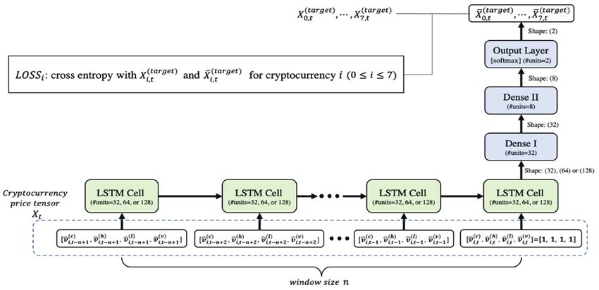
Fig. 2. Proposed LSTM model structure (windows size is and , = , ⊘ , , , = , ⊘ , ,
() () () ( ) ( ) ( )
, = , ⊘ , , , = , ⊘ , for 1 )
As shown in Fig. 2, our LSTM model consists of one LSTM layer having LSTM cells, two Dense
layers, and one output layer. For time epoch , price tensor is used for input for the LSTM layer. The
number of hidden units of an LSTM cell will be 32, 64, or 128. The proper number of units will be chosen
by the model tuning process and explained in the next subsection. On the other hand, the numbers of
hidden units at Dense I and II layers are fixed at 32, 8, and 2. Except for the last output layer using
“softmax,” all LSTM and other Dense I and II layers use the activation function selected by the model
tuning process, which will be explained in Section 4.2. Since the last output layer’s activation is “softmax,”
the output vector has only two values added up to 1, and they can be interpreted as probabilities for price
( ) ( )
up and down trends. For , the last outputs , are compared with target data , for
price tensor . For loss function , we use the cross entropy indicating the distance between
( ) ( )
, and , .
J Inf Process Syst, Vol.15, No.3, pp.694~706, June 2019 | 699Time Series Classification of Cryptocurrency Price Trend Based on a Recurrent LSTM Neural Network 4.2 Model Tuning A machine learning model has various hyper-parameters that determine the network structure (e.g., number of hidden units) as well as how the models are trained (e.g., type of optimizer). The performance of a model can vary considerably according to the selected set of hyper-parameters. In this study, we used the grid search method [14] to find the optimal hyper-parameters for our cryptocurrency price dataset by trying every possible combination of hyper-parameters based on the dataset. We also verified the validity of the model by performing k-fold cross-validation [15,16] in addition to finding the optimal hyper-parameters. To demonstrate the superiority of the proposed LSTM model, we also used the GB classifier model, which is known as a traditional machine learning model showing good performance in various fields [12,17]. The GB model is an ensemble learning model for prediction by combining outputs from individual trees. It builds trees one at a time, with each new tree helping correct the errors made by the previously trained tree. It exploits the boosting scheme, which focuses step by step on difficult data samples by strengthening the impact of the successful classification. For the purpose of fairness, we also performed the same model tuning process for the GB classifier model. Fig. 3. Overall model tuning process with grid search-based k-fold cross-validation. Fig. 3 shows the overall process of finding the optimal set of hyper-parameters and validating the GB and LSTM models with optimal ones. First, we separate the cryptocurrency price dataset into learning and test data. Next, -fold cross-validation based on grid search is performed. In -fold cross-validation, the training dataset is randomly partitioned into equal-sized sub-datasets. Among the sub-datasets, a single sub-dataset is retained as validation data for testing the model, and the remaining 1 sub- datasets are used as training data. The cross-validation process is then repeated times, with each of the sub-datasets used exactly once as validation data. The results can then be averaged to produce a single set of optimal hyper-parameters. The selected model is again trained by using the optimal hyper- parameters. Finally, the model performance is measured using the test data. The performance evaluation results are presented in Section 5. For the hyper-parameters of the LSTM model, we consider the following: (1) number of hidden units of an LSTM cell; (2) parameter initializer; (3) activation type; (4) dropout rate; and (5) optimization type. The number of hidden units of an LSTM cell is the dimensionality of the last output space of the LSTM 700 | J Inf Process Syst, Vol.15, No.3, pp.694~706, June 2019
Do-Hyung Kwon, Ju-Bong Kim, Ju-Sung Heo, Chan-Myung Kim, and Youn-Hee Han

layer. The parameter initializer represents the strategy for initializing the LSTM and Dense layers’ weight
values. The activation type represents the type of activation function that produces non-linear and limited
output signals inside the LSTM and Dense I and II layers. Furthermore, the dropout rate indicates the
fraction of the hidden units to be dropped for the transformation of the recurrent state in the LSTM layer.
Finally, the optimization type designates the optimization algorithm to tune the internal model
parameters so as to minimize the cross-entropy loss function. In the LSTM model, the candidate values
used to perform the grid search for the hyper-parameters are listed in Table 3. The table also lists an
example of the optimal hyper-parameter values found by our model tuning process.

Table 3. Candidate and optimal sets of hyper-parameters for the LSTM model
                                                                            Example of optimal hyper-parameter
    Hyper-parameter name              Hyper-parameter values
                                                                                values ( = and = )
 Number of hidden units                     {32, 64, 128}                                  128
   (LSTM cell)
 Parameter initializer                  {normal, he_normal,                                  Normal
                                          glorot_normal}
 Activation type                        {relu, tanh, sigmoid}                                 Tanh
 Dropout rate                            {0.0, 0.2, 0.3, 0.4}                                     0.0
 Optimization type                   {SGD, RMSProp, Adagrad,
                                                                                            RMSProp
                                             Adam}

  On the other hand, Table 4 shows the candidate values used to perform grid search for the GB hyper-
parameters and also lists the optimal hyper-parameter values. For the GB model, we consider the
following: (1) maximum depth; (2) maximum features; (3) number of estimators; (4) subsamples; and (5)
minimum samples for split. For the details of these hyper-parameters, refer to [17].

Table 4. Candidate and optimal sets of hyper-parameters for the GB model
                                                                          Example of optimal hyper-parameter
    Hyper-parameter name           Hyper-parameter values
                                                                              values ( = and = )
 maximum depth                              {4, 5, 6}                                     5
 maximum features                       {all, sqrt, log2}                                    sqrt
 number of estimators                    {50, 75, 100}                                       100
 subsamples                              {0.8, 0.9, 1.0}                                     0.9
 minimum samples for split                  {2, 3, 4}                                         2

5. Prediction Performance Evaluation
  In this section, we evaluate the performance of the LSTM model’s binary classification and compare
the LSTM model’s prediction performance against that of the GB model as evaluated in [12].

5.1 Evaluation Environment
 Our evaluation task was executed on Ubuntu 16.04 LTS with 32 GB RAM and two GPU cards (NVIDIA
GTX 1080Ti 11 GB). We used Tensorflow-GPU 1.8 and Keras 2.2.0 operated with Python 3.6. According

                                                            J Inf Process Syst, Vol.15, No.3, pp.694~706, June 2019 | 701
Time Series Classification of Cryptocurrency Price Trend Based on a Recurrent LSTM Neural Network
to the process shown in Fig. 4, the 3-fold cross-validated grid search is first performed for the
cryptocurrency price tensor data set (that is, k=3), and the optimal hyper-parameters are found through
each model tuning. The model training is performed using the derived optimal hyper-parameters listed
in Tables 3 and 4. For such model training, the number of learning epochs is set to 200.
Fig. 4. Performance comparison of the proposed LSTM model and the GB model [12] in terms of seven
cryptocurrencies and window size = 25, 50, and 75 (unit of time is fixed to 10).
5.2 Performance Metrics
An unambiguous and thorough way of presenting the prediction results of a deep learning model is to
use a confusion matrix. Table 5 is an example of the binary confusion matrix by the LSTM model
evaluation when the window size is 10. In the binary confusion matrix, true positive (TP) indicates cases
wherein both actual label (i.e., price-up) and model prediction are correctly positive. False negative (FN)
indicates cases wherein the actual label is positive but the model prediction is incorrectly negative (i.e.,
price-down). False positive (FP) indicates cases wherein the actual label is negative (i.e., not RDP) but the
model prediction is incorrectly positive. Finally, true negative (TN) indicates cases wherein both actual
label and model prediction are correctly negative.
Table 5. Example of binary confusion matrix for the LSTM model evaluation ( = 25 and = 10)
Predictive positive Predictive negative
Actual positive 3251 (TP) 3864 (FN)
Actual negative 1601 (FP) 1791 (TN)
As shown in Table 5, there is an imbalance in the number of actual target data—the number of actual
positives is 7115 (=3251+3864), whereas the number of actual negatives is 3392 (=1601+1791). The
accuracy measurement can be misleading when there is such an imbalance. A model can predict the target
of the majority for all predictions and achieve high classification accuracy, and the model loses its
usefulness. To overcome the problem of accuracy measurement, we compute additional measurements
to evaluate the LSTM and GB models: recall, precision, and f1-score [18]. They are defined by using the
confusion matrix as follows:
702 | J Inf Process Syst, Vol.15, No.3, pp.694~706, June 2019Do-Hyung Kwon, Ju-Bong Kim, Ju-Sung Heo, Chan-Myung Kim, and Youn-Hee Han
= (4)
= (5)
× ×
1 = (6)
The f1-score represents the harmonic mean of precision and recall and indicates the classification
performance of a model relatively accurately. It is expressed in the range of 0–1, where the best value is
1. We compute the recalls, precisions, and f1-scores, and then finally get a single f1-score measurement
for the performance evaluation of the LSTM and GB models.
5.3 Evaluation Results
The evaluation is performed to compare the performance of the LSTM and GB models and show the
superiority of the LSTM model for predicting the cryptocurrency price trend. The GB model is used in
[12], and we also evaluate the GB model’s performance according to [12]. Fig. 5 shows the comparison of
the f1-score values for the two models with the seven cryptocurrencies in terms of the window size of the
price tensor. It can be seen that the LSTM model is always better than the GB model for all
cryptocurrencies and the window sizes tested. The f1-score values of the LSTM model are between 0.63
and 0.68, whereas those of the GB model are between 0.59 and 0.63. It indicates that a performance
improvement of about 7% can be expected with the LSTM model.
Fig. 5. Performance comparison of the proposed LSTM model and the GB model [12] in terms of seven
cryptocurrencies and window size = 25, 50, and 75 (unit of time is fixed to 10).
As shown in Fig. 5, it is difficult to find the performance distribution tendency according to the window
size. The LSTM model best predicts the price trend when the window size is just 25 for BCH, DASH, and
ETC and 50 for XRP and LTC. For BTC and ETH, the prediction performance is highest when the
window size is 75. Still, we can know that a large amount of data with long window size does not guarantee
high performance. We can also deduce that DASH is the best cryptocurrency for the LSTM model to
predict the price trend.
J Inf Process Syst, Vol.15, No.3, pp.694~706, June 2019 | 703Time Series Classification of Cryptocurrency Price Trend Based on a Recurrent LSTM Neural Network Fig. 6 illustrates the comparison of the f1-score values for the LSTM and GB models with the seven cryptocurrencies in terms of unit of times. Similar to the results shown in Fig. 5, we can also know that the LSTM model is always better than the GB model for all cryptocurrencies and units of time tested. With the LSTM model, we can expect a performance improvement of about 7% compared to using the GB model. Fig. 6. Performance comparison of the proposed LSTM model and the GB model [12] in terms of seven cryptocurrencies and unit of times = 10, 30, and 60 (window size is fixed to 25). As shown in Fig. 6, it is also difficult to find the performance distribution tendency according to the unit of time. The LSTM model best predicts the price trend when the unit of time is just 10 for BTC, ETH, and BCH and 30 for XRP, DASH, and ETC. For LTC, the prediction performance is highest when the unit of time is 60. Finally, we can also know that DASH is the best cryptocurrency for the LSTM model to predict the price trend, followed by XRP. 6. Conclusion In this study, we applied the LSTM model to classify the cryptocurrency price time series. We collected historic cryptocurrency price time series data via Bithumb API, preprocessed them, and encoded the clean data into the three-dimensional price tensor. We also presented our LSTM model structure as well as how to use such price tensor as input data of the LSTM model. In particular, our model tuning scheme was provided to find the most suitable LSTM model parameters. The results of the prediction performance show that XRP and DASH are relatively predictable, whereas BCH is relatively hard to predict. Moreover, it can be seen that there is no significant difference in the prediction performance according to the window size and unit of time. We have also demonstrated that the LSTM model has a better f1-score than the GB model. Despite using a simple LSTM model, the average f1-score is approximately 0.68 for DASH, whereas the corresponding f1-score of the GB model is only about 0.63. Therefore, the LSTM model is relatively suitable when classifying the cryptocurrency time series data with high volatility. In future work, we plan to use additional features (e.g., mining hash rate) to build a better LSTM model so that the model raises the f1-score further. 704 | J Inf Process Syst, Vol.15, No.3, pp.694~706, June 2019
Do-Hyung Kwon, Ju-Bong Kim, Ju-Sung Heo, Chan-Myung Kim, and Youn-Hee Han

Acknowledgement
  This research was supported by the Basic Science Research Program (No. 2018R1A6A1A03025526)
and in part by the BK-21 plus program through the National Research Foundation of Korea (NRF)
funded by the Ministry of Education and supported in part by the Education and Research Promotion
Program of KOREATECH in 2018.

References
[1] W. M. Grove, D. H. Zald, B. S. Lebow, B. E. Snitz, and C. Nelson, “Clinical versus mechanical prediction: a
     meta-analysis,” Psychological Assessment, vol. 12, no. 1, pp. 19-30, 2000.
[2] E. Kita, M. Harada, and T. Mizuno, “Application of Bayesian network to stock price prediction,” Artificial
     Intelligence Research, vol. 1, no. 2, pp. 171-184, 2012.
[3] G. T. Nguyen and K. Kim, “A survey about consensus algorithms used in blockchain,” Journal of Information
     Processing Systems, vol. 14, no. 1, pp. 101-128, 2018.
[4] P. K. Sharma, S. Y. Moon, and J. H. Park, “Block-VN: a distributed blockchain based vehicular network
     architecture in smart city,” Journal of Information Processing Systems, vol. 13, no. 1, pp. 184-195, 2017.
[5] S. Nakamoto, “Bitcoin: a peer-to-peer electronic cash system,” 2008; https://bitcoin.org/en/bitcoin-paper.
[6] U. Rajput, F. Abbas, and H. Oh, “A solution towards eliminating transaction malleability in bitcoin,” Journal of
     Information Processing Systems, vol. 14, no. 4, pp. 837-850, 2018.
[7] H. Jang and J. Lee, “An empirical study on modeling and prediction of bitcoin prices with Bayesian neural
     networks based on blockchain information,” IEEE Access, vol. 6, pp. 5427-5437, 2017.
[8] J. C. B. Gamboa, “Deep learning for time-series analysis,” 2017; https://arxiv.org/abs/1701.01887.
[9] Y. B. Kim, J. G. Kim, W. Kim, J. H. Im, T. H. Kim, S. J. Kang, and C. H. Kim, “Predicting fluctuations in
     cryptocurrency transactions based on user comments and replies,” PloS One, vol. 11, no. 8, article no.
     e0161197, 2016.
[10] Z. Jiang, D. Xu, and J. Liang, “A deep reinforcement learning framework for the financial portfolio
     management problem,” 2017; https://arxiv.org/abs/1706.10059.
[11] A. Radityo, Q. Munajat, and I. Budi, “Prediction of bitcoin exchange rate to American dollar using artificial
     neural network methods,” in Proceedings of 2017 International Conference on Advanced Computer Science and
     Information Systems (ICACSIS), Bali, Indonesia, 2017, pp. 433-438.
[12] J. S. Heo, D. H. Kwon, J. B. Kim, Y. H. Han, and C. H. An, “Prediction of cryptocurrency price trend using
     gradient boosting,” KIPS Transactions on Software and Data Engineering, vol. 7, no. 10, pp. 387-396, 2018.
[13] S. Hochreiter and J. Schmidhuber, “Long short-term memory,” Neural Computation, vol. 9, no. 8, pp. 1735-
     1780, 1997.
[14] H. Larochelle, D. Erhan, A. Courville, J. Bergstra, and Y. Bengio, “An empirical evaluation of deep architectures
     on problems with many factors of variation,” in Proceedings of the 24th International Conference on Machine
     Learning, Corvalis, OR, 2007, pp. 473-480.
[15] R. Kohavi, “A study of cross-validation and bootstrap for accuracy estimation and model selection,” in
     Proceedings of the 14th International Joint Conference on Artificial Intelligence, San Francisco, CA, 1995, pp.
     1137-1145.
[16] T. Fushiki, “Estimation of prediction error by using K-fold cross-validation,” Statistics and Computing, vol. 21,
     no. 2, pp. 137-146, 2011.
[17] A. Natekin and A. Knoll, “Gradient boosting machines, a tutorial,” Frontiers in Neurorobotics, vol. 7, article no.
     21, 2013.
[18] D. M. W. Powers, “Evaluation: from precision, recall and F-measure to ROC, informedness, markedness and
     correlation,” Journal of Machine Learning Technologies, vol. 2, no. 1, pp. 37-63, 2011.

                                                            J Inf Process Syst, Vol.15, No.3, pp.694~706, June 2019 | 705
Time Series Classification of Cryptocurrency Price Trend Based on a Recurrent LSTM Neural Network
Do-Hyung Kwon https://orcid.org/0000-0002-5951-2081
He is receiving the M.S. degrees in Interdisciplinary Program in Creative Engineering
from Korea University of Technology and Education, Cheonan, Korea. His research
interest includes time series analysis using machine learning and deep learning, and
reinforcement learning across various domains, especially, device control.
Ju-Bong Kim https://orcid.org/0000-0001-6406-3092
He received B.S. and M.S. degrees in Computer Science and Engineering from Korea
University of Technology and Education, Cheonan, Korea, in 2017 and 2019,
respectively. Currently, he is PhD student in department of Computer Science and
Engineering from Korea University of Technology and Education. His research
interests include deep learning and reinforcement learning across various domains,
especially, device control and blockchain assets.
Ju-Sung Heo https://orcid.org/0000-0002-2486-9515
He received B.S. and M.S. degrees in School of Computer Science and Engineering
from Korea University of Technology and Education, Cheonan, Korea, in 2017 and
2019, respectively. Currently, he is a PhD student in Interdisciplinary Program in
Creative Engineering from Korea University of Technology and Education. His
research interests include deep learning and reinforcement learning across various
domains, especially, device control and blockchain assets.
Chan-Myung Kim https://orcid.org/0000-0002-5286-9854
He received the Ph.D. degree in applied physics from Korea University of Technology
and Education, Cheonan, Korea, in 2016. He was a software engineer at Thinkonweb,
Inc., in 2017. Currently, he works as a post-doctorate researcher in KOREATECH
Advanced Technology Research Center.
Youn-Hee Han https://orcid.org/0000-0002-5835-7972
He received B.S. degree in Mathematics from Korea University, Seoul, Korea, in 1996.
He received his M.S. and Ph.D. degrees in Computer Science and Engineering from
Korea University in 1998 and 2002, respectively. From March 4, 2002 to February 28,
2006, he was a senior researcher in the Next Generation Network Group of Samsung
Advanced Institute of Technology. Since March 2, 2006, he has been a Professor in the
School of Computer Science and Engineering at Korea University of Technology and
Education, Cheonan, Korea. His primary research interests include theory and
application of mobile computing, including protocol design and mathematical
analysis. Since 2002, his activities have focused on mobility management, media
independent handover, and cross-layer optimization for efficient mobility support. His
research topics also include mobile sensor/actuator networks, social network analysis,
and deep learning. He has published approximately 150 research papers on the theory
and application of mobile computing, and has filed 30 patents on ICT (Information
and Communication Technology) domain. He has been serving as an editor for Journal
of Information Processing Systems (JIPS) since August 2011. In addition, he has also
made several contributions in IETF and IEEE standardization, and served as the co-
chair of s working group in Korea TTA IPv6 Project Group.
706 | J Inf Process Syst, Vol.15, No.3, pp.694~706, June 2019You can also read