A data-science-driven short-term analysis of Amazon, Apple, Google, and Microsoft stocks
←
→
Page content transcription
If your browser does not render page correctly, please read the page content below
A data-science-driven short-term analysis of Amazon, Apple,
                                                                Google, and Microsoft stocks
arXiv:2107.14695v1 [q-fin.ST] 30 Jul 2021

                                                    Shubham Ekapure∗†, Nuruddin Jiruwala‡, Sohan Patnaik§, Indranil SenGupta¶

                                                                                           August 2, 2021

                                                                                               Abstract
                                                        In this paper, we implement a combination of technical analysis and machine/deep
                                                    learning-based analysis to build a trend classification model. The goal of the paper is
                                                    to apprehend short-term market movement, and incorporate it to improve the underlying
                                                    stochastic model. Also, the analysis presented in this paper can be implemented in a
                                                    model-independent fashion. We execute a data-science-driven technique that makes short-
                                                    term forecasts dependent on the price trends of current stock market data. Based on the
                                                    analysis, three different labels are generated for a data set: +1 (buy signal), 0 (hold signal),
                                                    or −1 (sell signal). We propose a detailed analysis of four major stocks- Amazon, Apple,
                                                    Google, and Microsoft. We implement various technical indicators to label the data set
                                                    according to the trend and train various models for trend estimation. Statistical analysis
                                                    of the outputs and classification results are obtained.

                                                Key Words: Short-term forecasting, stochastic model, feature extraction, classification
                                            results, LSTM.

                                            1       Introduction
                                            Stock market prediction is the act of trying to determine the future value of a company stock
                                            or other financial instrument traded on an exchange. The successful prediction of future price
                                            of a stock could yield significant profit. A long-term model for a stock is ambitious and may
                                            not be very realistic. However, there have been attempts to model the stock for a short-
                                            term. There has been a fair amount of research in this field and the prediction methodologies
                                            can be broadly classified into three categories- fundamental analysis, technical analysis, and
                                            machine/deep learning-based analysis.
                                                ∗
                                                 Author ordering is based on the alphabetical order of the last names. Contributions of the first three authors
                                            are equal. The last author is the research mentor of this REU project.
                                               †
                                                 Indian Institute of Technology Kharagpur, West Bengal, India
                                               ‡
                                                 Indian Institute of Technology Kharagpur, West Bengal, India
                                               §
                                                 Indian Institute of Technology Kharagpur, West Bengal, India
                                               ¶
                                                 Corresponding author. Associate Professor and Graduate Program Director, Department of Mathematics,
                                            North Dakota State University, Fargo, North Dakota, USA. Email: indranil.sengupta@ndsu.edu

                                                                                                    1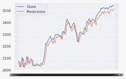
The fundamental analysis in the stock market aims to estimate the true values of the stock
price. After that, the stock price can be compared with its traded value on the stock markets.
Thus, this analysis finds out whether the stock on the market is undervalued or not (see [1]).
Finding out the true value can be performed by various methods with basically the same
principle. The principle is that a company is worth all of its future profits added together.
These future profits also must be discounted to their present value. This principle goes along
well with the theory that a business is all about profits and nothing else. As a matter of fact,
fundamental analysis is a long-term strategy that indeed, makes the stock trading decision
difficult in the short run. In the literature, the fundamental analysis is also implemented to
examine various financial statements with the aim to assess a real value of company’s stock.
The paper [3] provides a systematization of the fundamental analysis.
     Researchers, especially the short-term traders, are interested in the short-term forecasting
of the stock price and estimating the trend. Due to the dynamic nature and volatility in stock
price, even short-term prediction of the stock price becomes a challenging task. As technology
is continually improving, stock traders tend to move towards using intelligent trading systems
rather than fundamental analysis for predicting prices of stock. This helps the traders make
immediate investment decisions. This leads to the next two categories, technical analysis and
machine/deep learning-based analysis, mentioned above.
     The technical analysis seeks to determine the future price of stock based solely on the
trends of the past price (see [11]). Some of the common technical indicators that are used
to estimate the stock price movements are: exponential moving average (EMA), Bollinger
bands, moving average convergence divergence (MACD), momentum, volatility, RSI index etc.
Technical analysis is used for short-term strategy plans, therefore, making it relevant to the
field of short-term market prediction.
     Finally, in the category of machine/deep learning-based analysis, a good deal of meth-
ods are implemented in the recent literature. For example, in [9], certain index options are
constructed by efficient algorithms including uniform approximation error. In [7] the authors
study the optimal timing for an asset sale for an agent with a long position in a momentum
trade. In [10] a “deep momentum network” is introduced which is a hybrid approach that
incorporates deep learning-based trading rules into the volatility scaling framework of time
series momentum. The model also simultaneously learns both trend estimation and position
sizing from the empirical data. In [16] the authors propose a refinement of stock price dynamics
over some existing stochastic model. This refinement is obtained through the application of
data-science, especially machine/deep learning algorithms. This machine/deep learning-based
redefined model is implemented for commodity markets in [14, 15].
     In this paper, we implement a combination of technical analysis and machine/deep learning-
based analysis in order to build a trend classification model. That means, for the model and
analysis proposed in this paper, in addition to the robust artificial intelligence (AI) model, we
use technical indicators that capture the stock trend movement with greater accuracy. The
rest of the paper proceeds as follows. In Section 2, we provide a possible improvement of
the underlying stochastic model based on the data-science-driven short-term forecasting of
the stock prices. In Section 3, we provide a detailed description and perform exploratory data
analysis of the data sets that are considered for this paper. The methodology for a data-science-

                                               2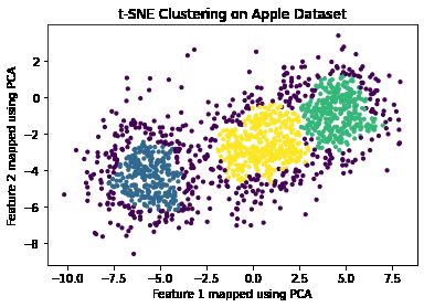
driven short-term forecasting is provided in Section 4. Statistical analysis of the outputs and
classification results are provided in Section 5. Finally, a brief conclusion is provided in Section
6. Some relevant statistical quantities for the data sets are provided in Appendix A.

2    Mathematical formulation
We assume that the share price St is given by

                      St = S0 eXt ,    where       dXt = bt dt + σt dWt + θt dJt ,             (2.1)

where bt is a deterministic function of t, Wt is the Brownian motions, and Jt is the jump
process with intensity λ. We assume that Wt and Jt , are independent. We write Jt in terms
of integral with respect to Poisson random measures N (dt, dx). Consequently,
                                              Z tZ
                                       Jt =             xN (dt, dx).
                                               0    R

Hence (2.1) can be written as
                                                                            Z
                          Xt
                 St = S0 e ,     where    dXt = bt dt + σt dBt + θt             xN (dt, dx).   (2.2)
                                                                            R

In addition to that, σt is assumed to be stochastic, and its dynamics are governed by

                                         dσt2 = F (σt2 , βt Ht )                               (2.3)

for an appropriate function F , where Ht is a jump process with intensity µ.
    There are some special cases of the proposed model that are studied in literature in con-
nection with the financial market, such as the Barndorff-Nielsen and Shephard (BN-S) model.
For the BN-S model, the share price (see , [4, 5, 13]) or commodity price (see, [17, 18]) St on
some risk-neutral probability space (Ω, G, (Gt )0≤t≤T , Q) is modeled by

                                          St = S0 exp(Xt ),                                    (2.4)
                                         1
                               dXt = (B − σt2 ) dt + σt dWt + ρ dZλt ,                         (2.5)
                                         2
                                  dσt2 = −λσt2 dt + dZλt ,       σ02 > 0,                      (2.6)
where the parameters B ∈ R, λ > 0 and ρ ≤ 0. In the above model, Wt is a Brownian
motion, and the process Zλt is a subordinator. Also W and Z are assumed to be independent,
and (Gt ) is assumed to be the usual augmentation of theR filtration generated by the pair
                                                               ∞
(W, Z). We consider a special case of (2.2), where dZs = ρ1 0 xN (ds, dx), is a subordinator.
Making   a scaling in the time variable, we define s = λt, for λ > 0. Then, we obtain, dZλt =
1 ∞
  R
ρ 0  xN   (λ dt, dx).

                                                     3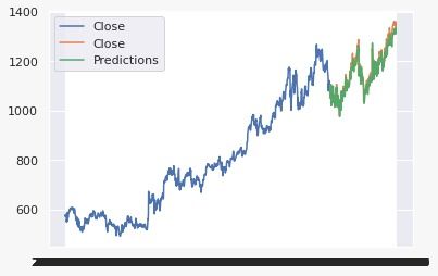
Since ρ ≤ 0, from (2.4) and (2.5), it is clear that the value of St primarily grows with
the drift coefficient B, and decays with the action of the subordinator Z. For a short-term
forecasting, we re-frame (2.5) as follows:
                                      1
                         dXt = (B(θ) − σt2 ) dt + σt dWt + ρ(θ) dZλt ,                    (2.7)
                                      2
where θ can take three values, 0 and ±1, and for an appropriate Λ ∈ R (obtained from data
calibration),
                                     (
                                       B,        if θ = 0, −1,
                              B(θ) =         2
                                                                                     (2.8)
                                       B + Λ , if θ = 1,
and                                       (
                                           ρ,       if θ = −1,
                                   ρ(θ) =                                                 (2.9)
                                           0,       if θ = 0, 1.
  Consequently, the indicator function θ, that provides a signal for the short-term share price
movement, can generate three scenarios:
Case 1: θ = 1, where a short-term upward share movement is expected:
                                            1
                             dXt = (B + Λ2 − σt2 ) dt + σt dWt .
                                            2
Case 2: θ = 0, where not much short-term share movement is expected:
                                          1
                                dXt = (B − σt2 ) dt + σt dWt .
                                          2
Case 3: θ = −1, where a short-term downward share movement is expected:
                                     1
                           dXt = (B − σt2 ) dt + σt dWt + ρ dZλt .
                                     2
In summary, the share price model, given by (2.4), (2.7), and (2.6), is driven by an indicator
function θ that can take values 1, 0, or −1, for short-term anticipated upward, stable or
downward share movements, respectively. For the rest of the paper, we derive a data-science
driven approach for finding the appropriate indicator function. In effect, the new model re-
frames and improves the classical BN-S model.

3     Data sets
We consider four stock data sets, viz. Amazon, Apple, Google, and Microsoft, to carry out
the statistical analysis. Training data sets are obtained between the years 2014 and 2019. For
testing, we consider intervals in the year 2021. Before executing the technical analysis on the
data, we perform exploratory data analysis on each of the data sets. Three approaches as
described below are primarily implemented for the basic data analysis. The primary objective

                                                4
is to get an estimation of the near-term stock fluctuation. For a model-independent analysis,
this is sufficient for a short-term investor to decide whether to sell, hold or buy a stock. From
the perspective of a stochastic model (i.e., for a model-dependent analysis), such estimation
will lead to the appropriate value of θ in (2.8) and (2.9).
• t-SNE Clustering Analysis: t-SNE clustering is a statistical method for visualizing
high-dimensional data by giving each data point a location in a two or three-dimensional
map. The idea behind t-SNE can be explained in simple terms: we are given with a set
x1 , ..., xn ∈ R, where x1 , x2 , . . . , are the feature vectors at a particular time step. These
multi-dimensional features are used for t-SNE clustering which maps them down to 2
dimensions using the principal component analysis (PCA). It is observed that the Google
stock data is clustered into two groups with some data points (outliers) outnumbered by
the other two clusters, whereas for Amazon, Apple, and Miscrosoft data, 3 prominent
clusters are found. The number of clusters can be thought of furnishing an intuition
regarding types of trends in the data. The time-series plot of Google data is somewhat
stable, and it keeps on increasing. This leads to the idea of two class labels- “increasing”
and “constant” (or, “stable”). For the other three data sets, three class labels can be
assigned corresponding to “increasing”, “constant” (or, “stable”), and “decreasing” stock
trends. Images of the Apple, Amazon, and Microsoft data sets, which are split into three
clusters are shown in Figure 1. In addition, the image of the Google data set which is
split into two clusters is shown in Figure 1.
Figure 1: t-SNE clustering for Apple, Amazon, Google, and Microsoft stocks.
5• Autocorrelation and correlation: Autocorrelation is a mathematical representation
of the degree of similarity between a given time series and a lagged version of itself over
successive time intervals. In all the stock data analysis for this paper, it is observed that
the stock prices have a high correlation with the near future prices. Intuitively, this gives
the idea that time series analysis models can be employed to estimate the stock price as
well as capture the trends. The auto-correlation plot for the Apple data is provided in
Figure 2. This shows that a high correlation is present when the lag is low (implying
strong dependence on near future stock prices).
Figure 2: Auto-Correlation plot for the Apple stock.
The autocorrelation plots for Amazon, Google and Microsoft stocks are shown in Figure
3, Figure 4, and Figure 5, respectively.
Figure 3: Auto-Correlation plot for the Amazon stock.
6Figure 4: Auto-Correlation plot for the Google stock.
Figure 5: Auto-Correlation plot for the Microsoft stock.
• PCA and Cosine Similarity: The multi-dimensional features are labeled +1 or −1
using the indicators that are mentioned in the subsequent methodology section. Once
the labeling of the data set is completed, the principal component analysis (PCA) is
implemented on the feature vectors followed by the computation of cosine similarity
between all the pairs of feature vectors in each of the classes of labels +1 and −1. It
is used to assess how different historical prices distribution vector are, and how related
the feature vectors are for their respective classes (i.e., +1 and −1). We also note that
the labels +1 and −1 in this context are the class labels of the stock trend- they do not
stand for the similar or dissimilar classes.
Various statistical quantities are computed for each of the four data sets on the attributes,
such as open price, high price, low price, close price, adjusted close price, volume SMA close,
EMA close, up, down, and RSI close. The results are provided in Appendix A.
74 Methodology
4.1 Feature extraction and label generation
The technical indicators can be broadly classified into four categories, viz. based on trend
indicator, momentum indicator, volume indicator, and volatility indicator. False signals arise
when a trader uses two or more indicators of the same category in order to make a trading
decision. For the technical analysis of this paper, we implement MACD which is based on the
trend indicator; RSI and TRIX which are based on the momentum indicator; and Bollinger
Bands which is based on the volatility indicator. Hence, our choice of indicators for the
classification pipelines successfully eliminates the false signal threat. The technical indicators
are briefly summarized below:
• MACD: The moving average convergence divergence (MACD) is a trend-following mo-
mentum indicator that shows the relationship between two moving averages of a security’s
price (see [2]). The MACD is calculated by subtracting the 26-period exponential moving
average (EMA) from the 12-period EMA. This causes MACD to oscillate around the zero
level. A signal line is created with a 9 period EMA of the MACD line. The formula for
calculating MACD is as follows:
MACD = EMA12 (C) − EMA26 (C), (4.1)
and
Signal Line = EMA9 (MACD), (4.2)
where C is the closing price, and EMAn is the n-day exponential moving average. We
consider the first instance of fall or rise of MACD line relative to the Signal Line, and
buy or sell accordingly. In other cases, we hold.
• RSI: The relative strength index (RSI) is a popular momentum indicator which de-
termines whether the stock is overbought or oversold (see [12]). A stock is said to be
overbought when the demand unjustifiably pushes the price upwards. In effect, this im-
plies that the stock is overvalued and should be sold. A stock is said to be oversold when
the price goes down sharply to a level below its true value. RSI ranges from 0 to 100
and generally, when RSI ≥ 70, it may indicate that the stock is overbought and when
RSI ≤ 30, it may indicate the stock is oversold. The formula for RSI is as follows:
1
RSI = 100 − , (4.3)
1 + RS
where
Average Gain Over past 14 days
RS = . (4.4)
Average Loss Over past 14 days
• TRIX: The triple exponential moving average oscillator (TRIX) is a momentum indi-
cator that oscillates around zero. It displays the percentage rate of change between two
triple smoothed exponential moving averages. The formula for TRIX is as follows:
EMA3 (i) − EMA3 (i − 1)
TRIX(i) = . (4.5)
EMA3 (i − 1)
8• Bollinger Bands: The Bollinger bands (BBANDS) study plots upper and lower enve-
lope bands around the price of the instrument (see [6]). The width of the bands is based
on the standard deviation of the closing prices from a moving average of price.
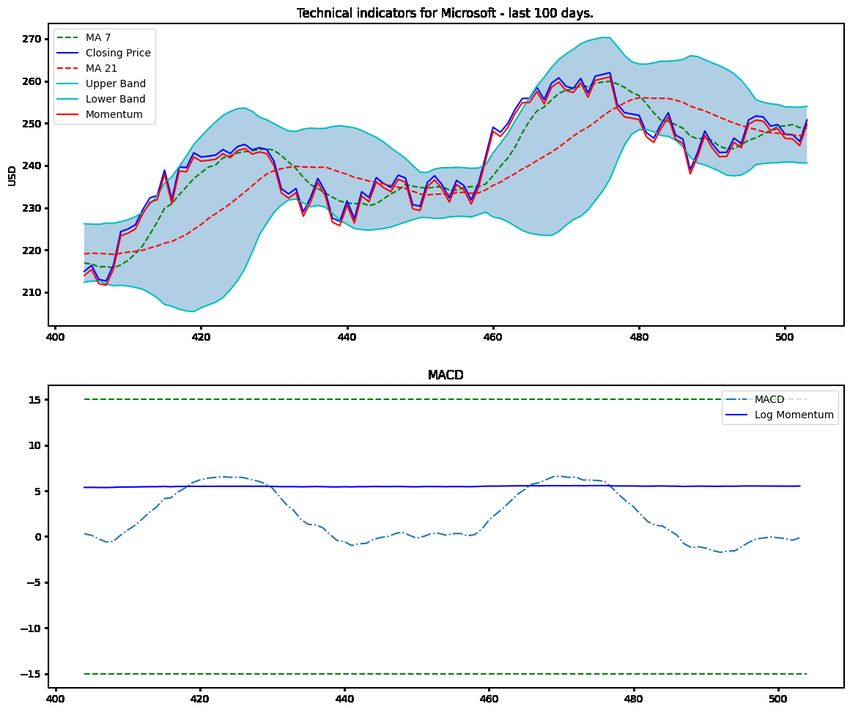
Figure 6 is the visualization of the plots of technical indicators such as 7 and 21 day moving
averages, closing price, upper and lower bands corresponding to Bollinger bands, momentum,
MACD and logarithmic mapping of momentum. The logarithmic mapping provides a fair
estimate of the stability of the stock time series data. Moreover, the Bollinger Bands provide
an intuition about the deviation of the stock from the simple moving average of the closing
price.
Figure 6: Plot of technical indicators on the Microsoft stock.
The four technical indicators mentioned above are implemented to generate the labels
(θ = 0, ±1) for the stock data sets.
• MACD: This indicator provides two outputs- MACD and MACD Signal Line (MACDSL).
The instance when the MACD crosses the MACDSL for the first time, it is considered a
sell (−1) signal, and for all consecutive instances when the MACD is above the MACDSL,
it is considered to be a hold (0). Similarly, the moment it drops below the MACDSL it is
considered to be a buy (+1) signal, and for all the following consecutive instances when
it is below MACDSL, it is considered to be a hold (0).
9• RSI: RSI close value ranges from 0 through 100. A value greater than 70 is considered
to be a sell (−1) signal, value less than 30 is considered to be a buy (+1) signal. If the
value lies in between 30 and 70, it is a hold (0) signal.
• TRIX: This indicator provides a single TRIX output that oscillates about zero line. The
instance when TRIX crosses the zero-signal line for the first time is considered to be a
sell (−1) signal, and for all consecutive instances when TRIX is above zero signal line, it
is considered to be a hold (0). Similarly, the moment it drops below zero signal line it is
considered to be a buy (+1) signal, and for all the following consecutive instances when
it is below zero signal line, it is considered to be a hold (0).
• Bollinger Bands: We get two outputs from this indicator: upper band (UBB) and
lower band (LBB). If the close value is greater than UBB, it is a sell (−1) signal, and if
the value is less than LBB it is a buy (+1) signal. If the close value is in between the
aforementioned two values, it is considered to be a hold (0).
The features used for time series forecasting are the values of close, momentum, and volatil-
ity. We use the latest 30 days data to generate 7 days of forecast. The indicator results and
their measures are used as features in the label classification pipeline, i.e., the classification
model is trained using indicator values as labels. The target for the final classification model
is generated by comparing the present value of close price (denoted by, close(t)) with the value
of close(t − 15), i.e., the close value 15 days ago. For our analysis, we sell (−1) if the difference
is positive and greater than 10% of close(t − 15). We buy (+1) if the difference is negative and
lesser than 10% of close(t−15). We hold (0) when the difference is between 0.1close(t−15) and
−0.1close(t − 15). This parameter for holding could be tuned based on the required margin
for the user. In summary,
θ = +1, if close(t) − close(t − 15) > 0.1close(t − 15), (4.6)
θ = 0, if − 0.1close(t − 15) ≤ (close(t) − close(t − 15)) ≤ 0.1close(t − 15), (4.7)
θ = −1, if close(t) − close(t − 15) < −0.1close(t − 15). (4.8)
4.2 Time series analysis
We implement the following analysis on the labels generated in the Subsection 4.1.
• ARIMA: ARIMA stands for AutoRegressive Integrated Moving Average which comes
under a class of model that captures a suite of different standard temporal structures in
time series data. We fit an ARIMA model on the stock data and observe that the closing
price is almost accurately predicted but there is a lag when there is a trend reversal of
the data. This is visualized in Figure 7 for the Microsoft data.
10Figure 7: ARIMA time series forecast on the Microsoft stock.
• LSTM: LSTM is one of the best time series prediction models. We use a single layer
network with only one epoch initially to check whether it can catch any trend. It is
observed that the values are not accurate, but it is able to capture the trend of the data.
With this motivation, we decide to use a two-layer LSTM with 25 epochs. The input is
30 days of close data, and the output is the predicted close value. Finally, we concatenate
and plot the close and predicted close values together. We find that the outputs are not
identical, but the model is able to capture the trend.
• LSTM (multiple features): In this setting, we use a multi feature LSTM to include
momentum, volatility, and close price of the stock data set. As more features are added,
more information is captured by the model and better forecasting is observed.
The mathematical equations behind LSTM are as follows. If Xt is the time series data,
we define
gt = tanh(Xt Wxg + ht−1 Whg + bg ),
it = σ(Xt Wxi + ht−1 Whi + bi ),
ft = σ(Xt Wxf + ht−1 Whf + bf ),
ot = σ(Xt Wxo + ht−1 Who + bo ),
ct = ft ct−1 + it gt ,
ht = ot tanh(ct ),
where is an element-wise multiplication operator, and, for all x = [x1 , x2 , . . . , xk ]> ∈ Rk
the two activation functions:
>
1 1
σ(x) = ,..., ] ,
1 + exp(−x1 ) 1 + exp(−xk )
11 >
1 − exp(−2x1 ) 1 − exp(−2xk )
tanh(x) = ,..., .
1 + exp(−2x1 ) 1 + exp(−2xk )
The Time Series Data plots for LSTM with multiple features are shown below.
In Figure 8, a multi-feature LSTM model, based on close price, momentum, and volatility,
is used to make a close price future forecast for the Microsoft stock. The blue and orange
labels indicate training and validation sets, respectively. The green label indicates forecasts
on validation set. In Figure 9, we observe the result on the Microsoft test set on a single day
window for the year 2021.
Figure 8: Multi-feature LSTM on the Microsoft train data.
Figure 9: Multi-feature LSTM on the Microsoft test data.
4.3 Predictive pipeline
On the generated outputs from Section 4.2, we perform label classification pipeline.
12• Random forest: Random forest is a supervised learning algorithm. It is an ensemble of
decision trees, usually trained with the “bagging” method, which is a combination of a
lot of machine learning models to improve the final decision. Based on the close forecast
generated for the next 7 days in the window, we predict the signal on them using the
supervised random forest classifier. The features in consideration are close, sign of moving
average convergence divergence, Bollinger bands, triple exponential average and relative
strength index. Also, the features associated with these indicators are also used. The
classifier is trained on the data of past 30 days.
• Boosted tree algorithms: Boosting means combining a learning algorithm in series
to achieve a strong learner from many sequentially connected weak learners. Trees in
boosting are weak learners but adding many trees in series and each focusing on the
errors from previous one make boosting a highly efficient and accurate model. There
are many ways of iteratively adding learners to minimize a loss function. Common
hyper-parameters for such models are maximum depth, maximum features, and minimum
samples per leaf.
• SVM: In machine learning, support-vector machine(SVM) is a supervised learning model
with associated learning algorithms that analyze data for classification and regression
analysis. SVM constructs a hyperplane or set of hyperplanes in a high-dimensional space,
which can be used for classification, regression, or other tasks like outliers’ detection.
Intuitively, a good separation is achieved by the hyperplane that has the largest distance
to the nearest training-data point of any class (so-called functional margin). In general,
the larger the margin, the lower the generalization error of the classifier.
The label classification model is based on a random forest classifier. There is a total of 13
features for the classification. We already know how the target variable is defined. The 13
features are close, 20-day simple moving average, and MACD measures (MACD sign, MACD
signal line, MACD actual line and the difference between signal line and actual line), Bollinger
Band measures (BB sign, Upper BB and lower BB), RSI measures (RSI sign, RSI close) and
TRIX measures (TRIX sign and TRIX line).
4.4 Architecture
In this subsection we combine the results in the Subsection 4.1, Subsection 4.2, and Subsection
4.3. We implement a LSTM based architecture to forecast the time series data. For this,
a classification model (for example, the random forest classifier) on top of the LSTM model
is implemented to estimate the trend class. The forecasting model has 3 LSTM layers and
a dense layer which provides the estimated time series data. This data is then fed into the
random forest classifier imported from sklearn (in Python) with the default hyper-parameter
setting for getting the class labels +1, 0, and −1. The architecture is schematically shown in
the Figure 10.
13Figure 10: Predictive pipeline architecture.
5 Analysis of the results
In this section, we propose certain tests in order to examine the goodness of fit of the forecasts
generated by the proposed model and architecture. After that, we evaluate the classification
task with some commonly used metrics.
5.1 Statistical Analysis
In order to check the goodness of fit, we used two tests- KS test, and KL divergence test. We
observe that the data generated by the architecture in Subsection 4.4 is a good estimated fit
to the original data.
• KS test: The Kolmogorov–Smirnov test (KS test) is a non-parametric test of the equality
of continuous, one-dimensional probability distributions that can be used to compare a
sample with a reference probability distribution (one-sample KS test), or to compare two
samples (two-sample KS test). We have used the test on our time series forecast to see
if the predictions and actual values of close come from the same distribution.
• KL divergence test: To measure the difference between two probability distributions
over the same variable X, a measure, called the Kullback-Leibler (KL) divergence test,
has been popularly used in the data mining literature. Here we assume that the original
distribution of time series data is P (x) and the predicted distribution is Q(x). For
14discrete probability distributions P and Q defined on the same probability space X, the
relative entropy from Q to P is defined as:
X P (x)
DKL (P ||Q) = P (x) log .
Q(x)
x∈X
The results of goodness of fit are shown in the Table 1 for all the four data sets.
Table 1: Goodness of fit.
Stock KS-Test (p-value) KL Div Test (entropy)
Apple 0.47 3.99e-05
Amazon 0.87 0.0001
Google 0.15 3.01e-05
Microsoft 0.99 6.54e-05
5.2 Classification results
• Weighted average F1-score: F1-score is a classification metric. It is calculated from
the precision and recall score for a case. Precision provides the relevance of the selection
and recall (also known as sensitivity) provides the number of relevant items considered.
For the weighted average F1-score, we calculate the F1-score for each label and obtain
the average considering the proportion for each label in the data set.
• Accuracy: Accuracy is also a common metric for evaluating classification models. It is
defined as the ratio of correct predictions over total prediction. An accurate model in a
classification model must be tested for its sensitivity for better generalization.
Based on the tree-based predictive model, we obtain the following result: 7-days forecast is
generated from the LSTM forecasting network using the previous 30-days of data. This method
is implemented to obtain predicted close prices for 4 windows, each of 7 days for June 2021.
This predicted close value is fed into the label classification pipeline. For all the stocks in our
consideration we obtain the accuracy and F1-scores. The results, shown in Table 2, seem to be
quite promising and consistent with the current benchmarks. These scores are the performance
value of the predictive model for coming up with an accurate call to hold, sell or buy the stock.
F1-score is measured to understand the general specificity of the model. A wrong prediction
may incur a lot of loss to the trader. Consequently, a good performance on both the aspects
is very important.
Table 2: Classification results.
Stock Accuracy F1-score
Apple 91.66 0.91
Amazon 95.8 0.95
Google 95.83 0.92
Microsoft 95.80 0.94
15Table 3 shows the accuracies and F1-scores on each of the features used (i.e., Bollinger
Bands, MACD, TRIX and RSI) for the four data sets (Microsoft (MSFT), Google (goog),
Apple (apple), and Amazon (amazon)).
Table 3: Accuracies and F1-scores on each of the features.
Tables 4, 5, 6, and 7 show the accuracies and F1-scores for different types for machine
learning classification model. To validate the final results more strongly we consider two
different test sets for testing out all the label classification algorithms. Tables 4 and 5 show
the results for the first test set from 02/22/21 (February 22, 2021) to 04/26/21 (April 26,
2021). Tables 6 and 7 show the results for the second test set from 04/27/21 (April 27, 2021)
to 06/25/21 (June 25, 2021).
Table 4: Accuracy results on test set 1: 02/22/21 to 04/26/21.
Data set Random Forest SVM Classifier XGB Classifier
Google test 88 90 79
Microsoft test 88 90 81
Amazon test 90 86 88
Apple test 85 86 82
Table 5: F1-score results on test set 1: 02/22/21 to 04/26/21.
Data set Random Forest SVM Classifier XGB Classifier
Google test 0.83 0.91 0.75
Microsoft test 0.83 0.91 0.83
Amazon test 0.86 0.84 0.85
Apple test 0.84 0.85 0.79
16Table 6: Accuracy results on test set 2: 04/27/21 to 06/25/21.
Data set Random Forest SVM Classifier XGB Classifier
Google test 98 97 97
Microsoft test 98 98 96
Amazon test 97 98 97
Apple test 93 98 93
Table 7: F1-score results on test set 2: 04/27/21 to 06/25/21.
Data set Random Forest SVM Classifier XGB Classifier
Google test 0.97 0.97 0.97
Microsoft test 0.98 0.98 0.97
Amazon test 0.97 0.97 0.97
Apple test 0.96 0.98 0.97
The analysis above corroborates the idea that the architecture proposed in the paper can
accurately capture the short-term movement of one of the four concerned stocks. This is
important for short-term traders. In addition, this also improves the underlying stochastic
model by finding the value of θ (0, or ±1) that can be implemented to (2.8) and (2.9). The
resulting model can be considered as an improved BN-S model.
6 Conclusion
In this work, we present a model that captures the trend for four different stock data sets,
namely, Amazon, Apple, Google, and Microsoft. A thorough exploratory data analysis gives
us an intuition of the data, and the hidden clusters provide us the idea about the three
classes- −1, 0, and +1. Furthermore, we incorporate momentum and volatility in stock market
analysis with deep learning-based forecasting, followed by the use of technical indicators based
on momentum, volatility, and trend for the trend classification task. The model proves to be
robust in predicting the direction of the stock movement. This is also validated from good
accuracy and F1-score. For all the data sets, our final accuracy lies in the range of 90-95% on
a 7-day prediction window. The p-values obtained from the KS test and the entropy of KL
divergence test also show the robustness of LSTM network employed for forecasting the time
series stock data.
For the future work, we consider using ensemble modeling for the classification pipeline
and experimenting with different neural network architectures. Moreover, in our future work
we plan to incorporate features like those extracted from sentiment analysis of the companies.
In addition, it may be possible that the analysis presented in the paper is implementable to
other stocks.
17A Appendix: statistical quantities for the data sets
• Amazon Data
Open High Low Close Adj Close Volume SMA close EMA close up down RSI close
mean 984.3 993.2 973.6 983.9 983.9 4.17e+06 983.5 979.2 6.51 -5.55 56.15
std 566.8 571.6 560.6 566.3 566.3 2.29e+06 565.5 564.4 12.81 12.99 16.81
min 284.4 290.4 284.0 286.9 286.9 8.81e+05 291.1 294.5 0.00 -139.35 11.43
25% 439.3 444.7 435.5 439.4 439.4 2.72e+06 439.5 435.8 0.00 -5.22 44.36
50% 818.0 821.6 812.5 817.8 817.8 3.56e+06 818.8 816.1 0.90 0.00 55.94
75% 1604.0 1622.7 1590.7 1602.9 1602.9 4.80e+08 1603.2 1600.4 8.16 0.00 68.25
max 2038.1 2050.5 2013.0 2039.5 2039.5 2.38e+07 2012.1 1985.2 128.51 0.00 93.97
• Apple Data
Open High Low Close Adj Close Volume SMA close EMA close up down RSI close
mean 35.98 36.29 35.67 35.99 34.20 1.61e+08 35.97 35.82 0.21 -0.17 56.46
std 11.64 11.74 11.55 11.66 12.03 9.06e+07 11.57 11.48 0.35 0.36 18.08
min 17.68 17.91 17.62 17.84 15.87 4.54e+07 17.92 18.45 0.00 -3.93 8.21
25% 26.96 27.21 26.70 26.98 24.89 1.01e+08 27.05 27.02 0.00 -0.20 43.06
50% 32.29 32.62 32.07 32.34 29.60 1.36e+08 32.30 32.05 0.02 0.00 56.77
75% 43.81 44.29 43.62 43.95 42.51 1.97e+08 43.92 43.64 0.31 0.00 69.88
max 72.77 73.49 72.02 72.87 72.02 1.06e+09 71.97 70.82 2.80 0.00 95.93
• Google Data
Open High Low Close Adj Close Volume SMA close EMA close up down RSI close
mean 854.1 861.3 846.7 854.2 854.2 1.83e+06 853.9 851.6 4.59 -4.07 54.43
std 248.3 250.6 246.5 248.7 248.7 1.06e+06 247.9 246.9 8.22 8.18 15.90
min 493.3 494.6 486.2 491.2 491.2 7.92e+03 496.1 503.4 0.00 -99.09 15.37
25% 601.6 604.1 595.4 599.6 599.6 1.23e+06 604.4 598.3 0.00 -5.13 42.90
50% 798.2 803.5 793.3 797.1 797.1 1.53e+06 798.8 792.9 0.42 0.00 53.79
75% 1083.5 1094.2 1073.4 1082.8 1082.8 2.05e+06 1083.4 1083.1 6.75 0.00 65.35
max 1363.3 1365.0 1352.7 1361.2 1361.2 1.11e+07 1354.9 1348.9 118.3 0.00 99.16
• Microsoft Data
Open High Low Close Adj Close Volume SMA close EMA close up down RSI close
mean 74.55 75.14 73.90 74.56 70.39 2.98e+07 74.50 74.17 0.40 -0.32 56.83
std 32.60 32.81 32.30 32.58 33.34 1.44e+07 32.43 32.27 0.72 0.69 15.06
min 34.73 35.88 34.63 34.98 30.11 7.42e+06 35.61 36.11 0.00 -6.09 15.71
25% 46.93 47.45 46.54 47.00 41.99 2.12e+07 46.94 46.73 0.00 -0.36 46.29
50% 62.70 63.08 62.27 62.63 58.45 2.66e+07 62.71 62.64 0.05 0.00 56.26
75% 101.1 101.8 99.51 101.1 97.39 3.40e+07 100.8 100.7 0.57 0.00 67.25
max 159.4 159.6 158.2 158.9 156.6 2.02e+08 158.0 156.5 6.59 0.00 99.11
18References
[1] J. Abarbanell, and B. Bushee (1997), Fundamental Analysis, Future Earnings, and Stock Prices, Journal
of Accounting Research, 35(1), 1-24.
[2] G. Appel (2005), Technical Analysis: Power Tools for Active Investors, publisher: FT Press.
[3] S. Baresa, S. Bogdan , and Z. Ivanovic, Zoran (2013), Strategy of stock valuation by fundamental analysis,
UTMS Journal of Economics, 4(1), 45-51.
[4] O. E. Barndorff-Nielsen and N. Shephard (2001), Non-Gaussian Ornstein-Uhlenbeck-based models and
some of their uses in financial economics, Journal of the Royal Statistical Society: Series B (Statistical
Methodology), 63, 167-241.
[5] O. E. Barndorff-Nielsen and N. Shephard (2001), Modelling by Lévy processes for financial econometrics, In
Lévy Processes: Theory and Applications (eds O. E. Barndorff-Nielsen, T. Mikosch & S. Resnick), 283-318,
Birkhäuser.
[6] J. A. Bollinger (2001), Bollinger on Bollinger Bands, publisher: McGraw-Hill Education.
[7] E. Ekström, C. Lindberg (2013), Optimal Closing of a Momentum Trade, Journal of Applied Probability,
50(2), 374-387.
[8] S. Habtemicael and I. SenGupta (2016), Pricing variance and volatility swaps for Barndorff-Nielsen and
Shephard process driven financial markets, International Journal of Financial Engineering, 3(4), 1650027
[35 pages].
[9] J. Jiang, W. Tian (2019), Semi-nonparametric approximation and index options, Annals of Finance, 15,
563-600.
[10] B. Lim, S. Zohren, and S. Roberts (2019), Enhancing Time-Series Momentum Strategies Using Deep Neural
Networks, The Journal of Financial Data Science, Fall 2019, https://doi.org/10.3905/jfds.2019.1.015.
[11] J. J. Murphy (1999), Technical Analysis of the Financial Markets: A Comprehensive Guide to Trading
Methods and Applications, publisher: New York Institute of Finance.
[12] J. J. Murphy (2009), The Visual Investor: How to Spot Market Trends,, publisher: Wiley; 2nd edition.
[13] E. Nicolato and E. Venardos (2003), Option Pricing in Stochastic Volatility Models of the Ornstein-
Uhlenbeck type, Mathematical Finance, 13, 445-466.
[14] M. Roberts and I. SenGupta (2020), Sequential hypothesis testing in machine learning, and crude oil price
jump size detection, Applied Mathematical Finance, 27 (5), 374-395.
[15] M. Roberts and I. SenGupta (2020), Infinitesimal generators for two-dimensional L´evy process-driven
hypothesis testing, Annals of Finance, 16 (1),121-139.
[16] I. SenGupta, W. Nganje and E. Hanson (2021), Refinements of Barndorff-Nielsen and Shephard model: an
analysis of crude oil price with machine learning, Annals of Data Science, 8(1), 39-55.
[17] I. SenGupta, W. Wilson and W. Nganje (2019), Barndorff-Nielsen and Shephard model: oil hedging with
variance swap and option, Mathematics and Financial Economics, 13 (2), 209-226.
[18] W. Wilson, W. Nganje , S. Gebresilasie, I. SenGupta (2019), Barndorff-Nielsen and Shephard model for
hedging energy with quantity risk, High Frequency, 2 (3-4), 202-214.
19You can also read