CONSUMER ATTENTION AND STOCK RETURNS - BY ØYVIND CHRISTENSEN AND MARVINA TURSUN - 2021 UIS BUSINESS SCHOOL - UIS BRAGE

Consumer attention and stock returns

 By Øyvind Christensen and Marvina Tursun

 2021
 UiS Business School

UNIVERSITY OF STAVANGER BUSINESS SCHOOL

 MASTER'S THESIS
STUDY PROGRAM: THIS THESIS HAS BEEN WRITTEN WITHIN THE
 FOLLOWING FIELD OF SPECIALIZATION:
Master of Science in Business Administration
 Applied Finance

 IS THE THESIS CONFIDENTIAL?
 (NB! Use the red form for confidential theses)

TITLE:

Consumer attention and stock returns

AUTHOR(S) SUPERVISOR:

 Peter Molnár

Candidate number: Name:

2054 Øyvind Christensen
………………… …………………………………….

2023 Marvina Tursun
………………… …………………………………….

Acknowledgements
We would like to thank our supervisor Peter Molnár, Associate Professor at the University of
Stavanger, Business school, for his valuable and excellent guidance. He has been very helpful and
gave us valuable discussions and constructive feedback. Additionally, we would like to thank our
family and friends for their support during these past busy months.

Abstract
We investigate whether consumers attention measured by Google searches for company’s names and
brands can predict stock returns, volatility and trading volume for smartphone and sporting goods
manufacturers. Existing research has utilized Google searches mainly as a measure of investor
attention (searches for tickers), while we consider two measures of consumer attention: Google
searches for company names and brands. We do not find either of these two attention measures to be
related to stock returns or volatility. On the other hand, increased attention predicts decreased trading
volume in the subsequent week, no matter whether we considered brand or company searches. We
further investigate sporting goods companies and smartphone companies separately and find that the
conclusions remain similar.

Table of Contents

ACKNOWLEDGEMENTS ...................................................................................................................................... I
ABSTRACT ............................................................................................................................................................. II
1. INTRODUCTION ................................................................................................................................................ 1
2. DATA ................................................................................................................................................................... 3
 2.1 KEYWORD SAMPLE SELECTION .............................................................................................................................. 3
 2.2 GOOGLE TRENDS .................................................................................................................................................... 4
 2.3 SEARCH VOLUME INDEX CONSTRUCTION ............................................................................................................... 5
 2.4 FINANCIAL DATA ..................................................................................................................................................... 6
 2.4.1 Stock return ..................................................................................................................................................... 7
 2.4.2 Abnormal stock return..................................................................................................................................... 7
 2.4.3 Volatility and variance..................................................................................................................................... 7
 2.4.4 Trading Volume ............................................................................................................................................... 8
 2.5 SUMMARY STATISTICS............................................................................................................................................. 9
3. METHODOLOGY ............................................................................................................................................. 10

 3.1 PANEL DATA REGRESSION MODEL AND EXAMINING PREDICTIVE POWER OF SVIS............................................. 10
 3.2 DESCRIPTIVE MODELS........................................................................................................................................... 10
 3.3 PREDICTIVE MODELS ............................................................................................................................................ 11
4. RESULTS........................................................................................................................................................... 12

 4.1 REGRESSION MODEL RESULTS FOR ASVI SEARCH TERMS .................................................................................. 13
 4.1.1 Abnormal return ............................................................................................................................................ 13
 4.1.2 Abnormal trading volume.............................................................................................................................. 15
 4.1.3 Volatility ......................................................................................................................................................... 17
 4.2 REGRESSION MODEL RESULTS FOR ASVI FOR SMARTPHONE AND SPORTING GOODS COMPANIES .................... 19
 4.2.1 Abnormal return ............................................................................................................................................ 19
 4.2.2 Abnormal trading volume.............................................................................................................................. 22
 4.2.3 Volatility ......................................................................................................................................................... 24
5. CONCLUSION .................................................................................................................................................. 26
REFERENCE LIST ............................................................................................................................................... 27
APPENDIX ............................................................................................................................................................ 28
 APPENDIX A: KEYWORDS ........................................................................................................................................... 28
 Table 23. Company names ...................................................................................................................................... 28
 Table 24. Brand specific keywords.......................................................................................................................... 28

1. Introduction
Information technology plays an important role in the development of various sectors of the economy.
Currently, the internet is utilized extensively by the users for several purposes, for instance, browsing
and collecting information, uploading new information, and most importantly, exploring trends.
Researchers have found that it is possible to use internet search data to predict economic statistics
since 2005 (Ettredge, Gerdes, & Karuga, 2005) and there have been several other studies that have
investigated internet searchers data in various fields. The cost associated with obtaining this data is
minor, while this data might become increasingly useful and easily accessible. Thus, the number of
searching for attention on internet increases day by day. Several search engines are available to users,
such as Yahoo, Bing, and Baidu, but the most frequently used search engine is Google.

Google search engine is the most popular search engine (Johnson, 2021). The search engine and its
analyzing tool Google Trends allow to access huge collections of various statistical data from
searches. Kulkarni, Haynes, Stough, and Paelinck (2009) found that Google data could improve
analyzing of economic activities, the level of accuracy and gives a better prediction for financial
forecasting. Data from Google Trends may be associated with present values of various economic
indicators such as automobile sales, unemployment requirements, travel purpose planning, and
consumer confidence (Choi & Varian, 2011) and it can be used for short-term economic forecasts.
Preis, Reith, and Stanley (2010) examined the connection between search volume data and market
changes. They found that weekly transaction volumes of S&P 500 firms correlate positively with the
weekly search volume of the company names and that the price changes influence search volumes in
the coming weeks.

In the finance field, Preis, Moat, and Stanley (2013) observed that Google Trend data consider
features of the current state of the economy and provide insight into future trends in the behavior of
economic aspects. Nevertheless, another research, such as Challet and Ayed (2014), confirmed that
random finance-related keywords are not reliable indicators of exploitable predictive information than
other random keywords. Da, Engelberg, and Gao (2011), Dimpfl and Jank (2016), and Goddard, Kita,
and Wang (2015) all employed multiple search terms such as company name, stock tickers, and other
terms used on stock exchanges, during the process of searching data and investigating the attention
of investors. Vlastakis and Markellos (2012) found that information demand directly affects the major
stock price fluctuations and trading volume of the thirty largest US stocks.

 1

One way to measure investors’ attention is to use Google and analyze the top search results. A
problem that may occur, is that companies can pay search engine optimization companies to get
higher up on search results. For this reason, investors can have excessive attention to the companies
who spends money on these activities which are more visible than non-promoted companies. Several
studies have been using search volume index (SVI) as a direct measure of investor attention to avoid
this problem. In the case of investment decisions and stock returns, the Google search engine grasps
the attention of investors, and it reduces the probability of asymmetric information. Since Google
Trends can capture real-time search trends, the data has also been used in other various applications,
such as influenza surveillance in South China (Kang, Zhong, He, Rutherford, & Yang, 2013) and
predicting sales, open numbers for movies, and ranking of songs (Goel, Hofman, Lahaie, Pennock,
& Watts, 2010). However, for economic research studies, Da et al. (2011) were among the first to
employ SVI as a measure of investor attention. They observe a positive relationship between SVI and
stock prices in the following weeks, in line with the results of Preis et al. (2010). Another study by
Joseph, Wintoki, and Zhang (2011) also used SVI as a measure of investor sentiment.

Nevertheless, most recent finance literature uses Google Trends as a measure of investor attention,
where they often use tickers as keywords. Tickers are the symbol for the publicly traded companies,
and sometimes they are not very descriptive. For instance, searching for the ticker “SAN” will give
all kinds of search results instead of their company name, Banco Santander. This is because “SAN”
has many different meanings. Bijl, Kringhaug, Molnár, and Sandvik (2016) found that a meaningful
and negative correlation exists between weekly abnormal search volumes and following stock returns.
They assume that company name searches have a more powerful relationship to stock market returns
than stock ticker searches. A recent study by Kim, Lučivjanská, Molnár, and Villa (2019) did not find
any evidence that Google searches could explain stock returns in the Norwegian stock market.
However, they found a relationship between Google searches and volatility and trading volume. We
complement the existing literature by using Google Trends to capture consumer attention, and
compare this with two consumer-related industries, smartphones, and sporting goods, but not related
to each other. We, therefore, use different keywords for the twenty companies we have selected to
analyze. For example, we have selected "Apple", "Xiaomi", "Adidas", and "Nike." The complete list
can be viewed in tables 1 and 2. By this, we study the correlation between consumer attention
represented by SVI from Google Trends and stock returns from Yahoo finance.

We chose two groups of companies: smartphone and sporting goods companies, because both of us
are interested in these businesses. The group of companies are consumer-related simply because
people are purchasing their products for their personal use. Users often like to have the latest
technology or latest trend. Moreover, sporting goods companies have different seasons where they

 2

launch new products, like smartphone companies, which launches new models each year. It will be
also interesting to see if our research will get similar results when comparing the two groups of
businesses, because it looks like there is no relationship between buying a smartphone and shoes.

The whole paper is organized as follows. Section 1, as we stated above, and Section 2 introduces the
data used in the paper. The methodology is defined in Section 3. Section 4 presents our findings and
a discussion of the results. We conclude in Section 5.

2. Data
In this section, we present our data sources and handling techniques we used. We construct five
variables, two attention variables measured by Google search volumes for company names and brand
names and volatility, abnormal stock return, abnormal trading volume. The Google search data is
representing consumer attention. We collected a dataset covering weekly data over a five-year period
from 2016 to 2020. We select two industries where brand names are important: smartphone producers
and producers of sport equipment.

2.1 Keyword sample selection
First, we have looked at sales statistics and found some of the top smartphone and sporting goods
companies globally. These companies are some of the more popular in the world. This means they
will get attention from consumers and investors all over the world. If we would have selected smaller
companies, they might only sell their products in their local market. This could mean they would not
get the same attention from consumers abroad. We have selected the following twenty companies:
Apple, an American company, Blackberry from Canada, Nokia from Finland, LG and Samsung from
South Korea, Sony from Japan, ASUSTeK (Asus) and HTC from Taiwan, and Lenovo and Xiaomi
from China. We have selected these sporting goods companies: Nike, Lululemon, Under Armour,
Skechers, and Columbia from the United States, Adidas and Puma from Germany, Fila from South
Korea, and Anta from China.

The search categories we selected were company and brand categories. It is more likely consumers
know the company names and products, than company’s stock ticker. For example, for Blackberry,
searching for the ticker name “BB” would give to many results not related to the company Blackberry.
Most consumers are not professional investors who knows the different ticker names. With the help
of Google AdWords, we figured out which keywords are most relevant in the brand categories we
selected. The way Google AdWords keyword platform works, is that we input the company name
that we want to investigate, and it displays all relevant keywords with the time horizon and location
 3

we selected. Since the companies are located all over the world, we focus on search results from
worldwide Google search results. We reduced the number of keywords manually down to 10-15 most
relevant words per company. The reason for the reduction of the brand keywords is that including
keywords that are not very relevant would create too much noise.

We have the following two categories:

 1. Brand-related: incorporates the keywords by their brand names. For example, a brand name
 for Apple and Nike will have keywords which is constructed by their products and services,
 “iPhone 11”, “Apple Watch”, “Nike Air”, “Jordan 1”. This will be referred to as SV ! .
 2. Company-related: incorporates their company names as keywords. “Apple”, “Puma”,
 “Xiaomi” will be referred to as SV " .

The complete list can be found in the Appendix A.

2.2 Google Trends
Google Trends is an analyzing website created by Google to rank the most popular search queries
worldwide. It displays the search term frequency based on keywords and a given period called search
volume index (SVI). Each search is divided by total search for geography and time range. And then
normalized on a scale of 0-100.

The first step is to enter the brand name we have selected on a website called Google AdWords. Here
it is possible to see which other keywords are relevant for the brand name entered and it is ranked by
popularity. Then we reduced the relevant keyword sample from the Google AdWords platform to
around 10-15 brand-related keywords per company and used Google Trends to see how many search
hits each keyword has, and this is the raw SVI from Google Trends. To make the data clean as
possible, we exclude the keywords irrelevant for the companies and keywords with zero hits. (Preis
et al., 2013) mentioned that local investors prefer domestic market, and that global search volume
data are less successful than U.S. searches for the U.S. markets. The search results we have are based
on worldwide Google searches since the companies we have selected are located all over the world
and their products are being sold worldwide.

 4

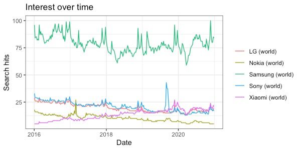
2.3 Search volume index construction
The SVI from Google Trends is an index with a scale from 0 to 100. The 100 represents the largest
share of the total queries in the chosen region for a search term (Choi & Varian, 2011). We standardize
SVI, to abnormal search volume index (ASVI) due to the nature of the type of regression and because
the companies in our sample vary a lot concerning trading volumes and the SVI. The two figures
below are graphs of SVI which shows the search trend for some of the company names we have
selected over the time period 2016-2020.

 Figure 1. Google Search Volume index for LG, Nokia, Samsung, Sony, Xiaomi between 2016 and 2020.

We focus on specific company names and brands as search terms but select the top-rated words to fit
more efficiently. Preis et al. (2010) found a relationship between Google Trend data for company
names and the transaction volumes of the identical stock on a weekly time range. All the company
names, and brands we search for, and keyword lists from Google AdWords are attached in the
appendix. To achieve more comparability among the companies we converted the raw SVI data to an
abnormal SVI (ASVI).

The method we used to standardize the SVI into ASVI, is taking the log of current week minus the
log median SVI during the previous eight weeks. We used the following formula for abnormal SVI
(Da et al., 2011):

 # = log # − log [ 3 #$%,… #$( 4] (1)

 5

2.4 Financial data
To study if there is a relationship between stock trading activity and consumer attention, we used
Yahoo Finance to download stock data for our selected companies, as well as their benchmark indexes
to calculate abnormal returns. Yahoo Finance provide Open, High, Low, Close, Adjusted Close and
Volume as daily data. We gathered data for five years. Furthermore, financial data are converted to
weekly data to match the data from Google Trends. For the risk-free rate calculations, we are using
the 10-year US Treasury constant maturity rate, which is used for the abnormal return calculations
based on Capital Asset Pricing Model (CAPM). The period is the same 2016-2020 and we are using
the average rate. The stock data downloaded is used to find abnormal trading volume, volatility, stock
prices, and index prices. The companies we have selected in our study are publicly traded companies
in stock markets around the world. We have used the following ten stocks and indexes for a period
of five years from 2016 to 2020:

Table 1. List of smartphone companies and their benchmark indices.

 Company name Stock ticker Index name Index ticker
 Apple Inc. AAPL S&P 500 ^GSPC
 Samsung Electronics Co Ltd 005930.KS Kospi Composite Index ^KS11
 Xioami Corp. 1810.HK Hang Seng Index ^HSI
 Sony Group Corp. 6758.T Nikkei 225 ^N225
 ASUSTeK Computer Inc. (ASUS) 2357.TW TSEC weighted index ^TWII
 Blackberry Limited BB.TO S&P/TSX Composite index ^GSPTSE
 Lenovo Group Limited 0992.HK Hang Seng Index ^HSI
 LG Electronic Inc. 066570.KS Kospi Composite Index ^KS11
 Nokia Corporation Nokia.HE OMX Helsinki 25 index ^OMXH25
 HTC Corp 2498.TW TSEC weighted index ^TWII

 6

Table 2. List of sporting goods companies and their benchmark indices.

 Company name Stock ticker Index name Index ticker
 Nike Inc. NKE Dow Jones Industrial Average ^DJI
 Adidas AG ADS.DE DAX Performance Index ^GDAXI
 Puma SE PUM.DE DAX Performance Index ^GDAXI
 Asics Corp 7936.T Nikkei 225 ^N225
 Under Armour Inc. UA Dow Jones Industrial Average ^DJI
 Lululemon Athletica Inc LULU NASDAQ 100 Index NDX
 Columbia Sportswear Company COLM NASDAQ 100 Index NDX
 FILA Holdings Corporation 081660.KS Kospi Composite Index ^KS11
 Skechers U.S.A., Inc. SKX Dow Jones Industrial Average ^DJI
 ANTA Sports Products Limited 2020.HK Hang Seng Index ^HSI

2.4.1 Stock return
We use the adjusted return calculated from Yahoo Finance, since it is adjusted for stock splits and
dividend distributions calculated the following way:

 #
 # = log 7 ; (2)
 #$%

where # is the stock return and # is adjusted stock price for the week t.

2.4.2 Abnormal stock return
For finding the abnormal return, we are use Capital Asset Pricing model (CAPM):

 ) = ) − ) ∗ 3 * − + 4 − + (3)

Where ri is the stock return of company i, rf is the risk-free rate calculated as a mean of 2016-2020 of
the US 10-Year Treasury Constant Maturity Rate and βi is the company’s beta.

2.4.3 Volatility and variance
Volatility is a standard measure to evaluate how stock returns fluctuate over time. (Parkinson, 1980)
was the first to improve this method by implementing high and low price instead of closing price. But
then Garman and Klass (1980) improved it again by adding opening and close price. We use one with
a further improvement for estimating volatility utilizing volatility estimator adjusted for the opening
jump, as discussed by Molnár (2012) The information used from Yahoo Finance is the open, high,
 7

low, close, and adjusted close prices during a trading day t to calculate the volatility for the current
day in the following way:

 # = log( ) − log( ) (4)

 # = log( ) − log( ) (5)

 ℎ# = log(ℎ ℎ ) − log( ) (6)

 # = log( ) − log ( )#$% (7)

Opening jump adjusted equation:

 # = log( ) − log ( )#$% (8)

 # = log( . ) − log ( . )#$% (9)

 #
 # = # ∗ (10)
 #

First, we calculate the daily variance with following formula:

 1
 # = (ℎ − # ), − (2 2 − 1) # , + #, (11)
 2 #

The next step is calculating the weekly volatility as a square root of average daily variance from a
specific week:

 1
 # = W Y # (12)
 | # |
 )∈.!

Where S is the set of trading days in a specific week t.

2.4.4 Trading Volume
The weekly trading volume is calculated as an average of daily trading volumes from a specific week:

 1
 # = Y # (13)
 | # |
 )∈.!

Where S is the set of trading days in a specific week t.

 8

The abnormal weekly trading volume is calculated as follows:

 1
 # − 52 ∑/,
 )0% #$)
 # = (14)
 12!

Where # is abnormal trading volume, # is trading volume and 12! is the standard deviation of
the trading volume.

2.5 Summary statistics

Table 3. Descriptive statistics for all variables

 Descriptive Statistics
 N Mean St. dev. Min Max Skew Kurtosis

 345 4675.00 0.00 0.04 -0.35 0.35 0.00 7.58
 #! 4675.00 -0.01 0.20 -2.06 1.12 -1.80 15.23
 #" 4675.00 -0.00 0.13 -1.59 1.14 -0.38 22.95
 # 4675.00 -4.54 4.00 -53.03 5.25 -2.78 22.30
 # 4675.00 0.08 0.13 0.01 2.34 6.04 60.16

In table 3 we present the summary table for all the variable that we created from our raw data. The
abnormal stock returns are calculated from the CAPM addressed in section “stock return” The ASVI
is based on search terms calculated using Da et al. (2011) formula with an eight-week median time
horizon explained in the section “Google Trend.” Volatility is constructed by using the weekly Jump
adjusted Garman-Klass. The abnormal trading volume is calculated from the formula Zheng (2007)
as we addressed in “Trading volume.”

Table 4. Correlation Matrix for variables

 Correlation Matrix
 #345 #! #" # #
 #345 1
 #! 0.003 1
 #" -0.004 0.558 1
 # 0.001 -0.094 -0.058 1
 # 0.005 -0.041 -0.023 0.117 1

 9

In table 4 we study the correlation between the variables to evaluate whether consumer attention
(company and brand) can provide additional information to the information provided by the other
variables. The correlation matrix reported in table 4 shows a small correlation coefficient among the
consumer attention (ASVI) and the other variables, as the correlation coefficients are all close to
zero. When comparing both ASVI together, there is a correlation at 0.558. Which means they have
a connection with some search words.

3. Methodology
In this section, we will describe the models and equations used to investigate our main research,
whether there is a relation between consumer attention and stock returns. Simultaneously, we
examined the other variables: abnormal trading volume and volatility. We present the panel data
regression model in 3.1, the descriptive model in 3.2, and lastly, the predictive model in 3.3.

3.1 Panel data regression model and examining predictive power of SVIs.
We investigate whether stock returns are explained or predicted by an ASVI, volatility, or abnormal
trading volume utilizing the panel data regressions with fixed effects. All regression models included
a lagged dependent variable. Since we want to examine which ASVI variable is more significant in
the explaining and predicting return, we estimate the descriptive and predictive models with both
ASVI against with other variables.

3.2 Descriptive models
We estimate the following regression:

 #345 = + % #$%
 345
 + # (15)

 #345 = + % #$%
 345
 + , #! + # (16)

 #345 = + % #$%
 345
 + , #" + # (17)

 #345 = + % #$%
 345
 + , # + # (18)

 #345 = + % #$%
 345
 + , # + # (19)

 #345 = + % #$%
 345
 + , #! + 6 # + 7 # + # (20)

 #345 = + % #$%
 345
 + , #" + 6 # + 7 # + # (21)

 #345 = + % #$%
 345
 + , #! + 6 #" + 7 # + / # + # (22)
 10

Previous studies and results by Da et al. (2011) motivated us to investigate and create a descriptive
model of trading volume on whether ASVI as a measurement of consumer attention can explain or
predict abnormal return since their study was focused on investor attention. The weekly abnormal
trading volume is used as a dependent variable to examine changes in trading volume are explained
by changes in search interest. We additionally include volatility, abnormal return, and lagged
abnormal trading volume as control variables. This results in the following regression model.

 # = + % #$% + , #! + 6 #" + 7 # + / #345 + # (23)

Next, we study whether there is an additional association between ASVI and volatility. We have
used the descriptive model below:

 # = + % #$% + , #! + 6 #" + 7 #345 + / # + # (24)

3.3 Predictive models
To see if is possible to forecast or predict abnormal return, we have created several models. In these
models, all explanatory variables are lagged from the previous week. These models are estimated as
panel data regressions with fixed effects. We first estimate them for the group of all companies
together, and later separately for smartphone companies and for sports equipment companies.

 #345 399 = + % #$%
 345 !
 + , #$% "
 + 6 #$% + 7 #$% + / #$% + # (25)

 #399 = + , #$%
 ! "
 + 6 #$% 345
 + 7 #$% + / #$% + + # (26)

 #399 = + + , #$%
 ! "
 + 6 #$% 345
 + 7 #$% + / #$% + # (27)

 11

4. Results
We used Heteroscedasticity-consistent standard errors in our models to control for possible
heteroskedasticity. All the results are presented with robust standard error. We organize this section
by presenting and discussing the results for both sporting goods companies and smartphones
companies together in section 4.1. We compare the regression results for sporting goods companies
and one for smartphone companies separately in section 4.2.

 12

4.1 Regression model results for ASVI search terms

4.1.1 Abnormal return

Table 5. Explanatory model
 Dependent variable: Abnormal Return
 (1) (2) (3) (4) (5) (6) (7) (8)
 $%& -0.052** -0.052** -0.052** -0.052**
 !"#
 (0.019) (0.019) (0.019) (0.019)
 !' 0.001 0.003 0.004
 (0.003) (0.003) (0.004)
 !( -0.001 0.0003 -0.003
 (0.005) (0.005) (0.006)
 ! 0.001 0.002 0.002 0.002
 (0.004) (0.004) (0.004) (0.004)
 ! 0.00001 -0.00001 -0.00001 -0.00001
 (0.0001) (0.0001) (0.0001) (0.0001)
Observations 4,657 4,675 4,675 4,675 4,675 4,657 4,657 4,657
R2 0.003 0.00001 0.00001 0.00002 0.00000 0.003 0.003 0.003
Adjusted R2 0.003 -0.0002 -0.0002 -0.0002 -0.0002 0.002 0.002 0.002

Note: Column (6) presents results from regression including all variables except ASVI Company, and column (7)
presents results from regression including all variables except ASVI Brand. And column (8) presents results from
regression including all variables. Robust standard errors are in parentheses. The sample period covers weekly data
from 2016 to 2020. The symbols ** and * denote significance at the 1% and 5% levels, respectively.

Table 6. Predictive model
 Dependent variable: Abnormal Return
 (1) (2) (3) (4) (5) (6) (7) (8)
 $%&
 !"# -0.052** -0.052** -0.052** -0.052**
 (0.019) (0.019) (0.019) (0.019)
 '
 !"# 0.003 0.003 0.004
 (0.003) (0.003) (0.004)
 (
 !"# -0.0001 -0.001 -0.004
 (0.005) (0.005) (0.006)
 !"# -0.009* -0.008* -0.009* -0.008*
 (0.004) (0.004) (0.004) (0.004)
 !"# -0.0001 -0.0001 -0.0001 -0.0001
 (0.0001) (0.0001) (0.0001) (0.0001)
Observations 4,657 4,657 4,657 4,657 4,657 4,657 4,657 4,657
R2 0.003 0.0002 0.00000 0.001 0.0001 0.004 0.004 0.004
Adjusted R2 0.003 -0.00003 -0.0002 0.001 -0.0001 0.003 0.003 0.003

Note: Column (6) presents results from regression including all variables except ASVI Company, and column (7)
presents results from regression including all variables except ASVI Brand. And column (8) presents results from
regression including all variables. Robust standard errors are in parentheses. The sample period covers weekly data
from 2016 to 2020. The symbols ** and * denote significance at the 1% and 5% levels, respectively.

 13

Tables 5 and 6 present the results from the regressions on abnormal return using the weekly ASVI
company and brand as independent variables, together with volatility and abnormal trading volume.
With these models, we want to investigate the impact of consumer attention and the difference
between ASVI company and the ASVI brand, to see which one has stronger impact on abnormal
returns. We conclude that the weekly ASVI for both company and brand can neither explain nor
predict the abnormal return. However, there is a negative association between previous abnormal
return and current abnormal return in both models. For table 6, the lagged volatility can predict the
abnormal return in the single and all three multiple regressions. The magnitude of this relationship is
very small, as documented by small regression coefficient and low regression’s R2.

 14

4.1.2 Abnormal trading volume

Table 7. Explanatory model
 Dependent variable: Abnormal trading volume
 (1) (2) (3) (4) (5) (6) (7) (8)
 !"# 0.841** 0.837** 0.838** 0.837**
 (0.033) (0.033) (0.033) (0.033)
 !' -1.895** -0.297* -0.210
 (0.236) (0.143) (0.168)
 !( -1.748** -0.411 -0.239
 (0.437) (0.218) (0.256)
 ! 3.586** 0.694* 0.694* 0.692*
 (0.424) (0.288) (0.288) (0.288)
 !$%& 0.059 0.931 0.916 0.926
 (1.281) (0.811) (0.812) (0.811)
Observations 4,657 4,675 4,675 4,675 4,675 4,657 4,657 4,657
R2 0.702 0.009 0.003 0.014 0.0000 0.703 0.703 0.703
Adjusted R2 0.702 0.009 0.003 0.013 -0.0002 0.703 0.703 0.703

Note: Column (6) presents results from regression including all variables except ASVI Company, and column (7)
presents results from regression including all variables except ASVI Brand. And column (8) presents results from
regression including all variables. Robust standard errors are in parentheses. The sample period covers weekly
data from 2016 to 2020. The symbols ** and * denote significance at the 1% and 5% levels, respectively.

Table 8. Predictive model
 Dependent variable: Abnormal trading volume
 (1) (2) (3) (4) (5) (6) (7) (8)
 !"# 0.841** 0.834** 0.836** 0.834**
 (0.033) (0.033) (0.033) (0.033)
 '
 !"# -2.253** -0.645** -0.548**
 (0.240) (0.146) (0.173)
 (
 !"# -2.178** -0.717** -0.261
 (0.421) (0.199) (0.235)
 !"# 3.885** 0.904** 0.922** 0.904**
 (0.452) (0.272) (0.271) (0.272)
 $%&
 !"# -1.178 -1.137 -1.155 -1.141
 (1.223) (0.633) (0.635) (0.634)
Observations 4,657 4,675 4,675 4,675 4,675 4,657 4,657 4,657
R2 0.702 0.009 0.003 0.014 0.0000 0.703 0.703 0.703
Adjusted R2 0.702 0.009 0.003 0.013 -0.0002 0.703 0.703 0.703

Note: Column (6) presents results from regression including all variables except ASVI Company, and column (7)
presents results from regression including all variables except ASVI Brand. And column (8) presents results from
regression including all variables. Robust standard errors are in parentheses. The sample period covers weekly
data from 2016 to 2020. The symbols ** and * denote significance at the 1% and 5% levels, respectively.

 15

We did not find any relationship between stock returns and ASVI. Next, we look further at the impact
of ASVI on other variables. We conduct similar regressions as we did with the abnormal return.
Tables 7 and 8 present the results from the abnormal trading volume with the same explanatory
variables. Since there is a positive relationship between volatility and abnormal trading volume,
therefore abnormal trading volume has the highest impact on volatility. These results are similar to
the results from the predictive model. We further observe a positive association between current and
previous abnormal trading volume in both regression models, and the two different ASVI can predict
abnormal trading volume.

 16

4.1.3 Volatility

 Table 9. Explanatory model
 Dependent variable: Volatility
 (1) (2) (3) (4) (5) (6) (7) (8)
 !"# 0.268** 0.259** 0.259** 0.259**
 (0.034) (0.034) (0.034) (0.034)
 !' -0.027* -0.004 0.0002
 (0.012) (0.009) (0.011)
 !( -0.023 -0.012 -0.012
 (0.014) (0.015) (0.017)
 $%& 0.014 0.038 0.038 0.038
 (0.035) (0.033) (0.033) (0.033)
 ! 0.004** 0.002** 0.002** 0.002**
 (0.0005) (0.0004) (0.0004) (0.0004)
 Observations 4,657 4,675 4,675 4,675 4,675 4,657 4,657 4,657
 R2 0.077 0.002 0.001 0.00002 0.014 0.084 0.084 0.084
 Adjusted R2 0.077 0.001 0.0003 -0.0002 0.013 0.083 0.083 0.083

 Note: Column (6) presents results from regression including all variables except ASVI Company, and column (7)
 presents results from regression including all variables except ASVI Brand. And column (8) presents results from
 regression including all variables. Robust standard errors are in parentheses. The sample period covers weekly data from
 2016 to 2020. The symbols ** and * denote significance at the 1% and 5% levels, respectively.

 Table 10. Predictive model
 Dependent variable: Volatility
 (1) (2) (3) (4) (5) (6) (7) (8)
 !"# 0.268** 0.260** 0.259** 0.260**
 (0.034) (0.034) (0.034) (0.034)
 ' -0.011 0.001 0.004
 !"#
 (0.009) (0.009) (0.010)
 ( -0.015 -0.005 -0.008
 !"#
 (0.015) (0.015) (0.018)
 $%& -0.014 -0.017 -0.017 -0.017
 !"#
 (0.036) (0.035) (0.035) (0.035)
 !"# 0.003** 0.002** 0.002** 0.002**
 (0.001) (0.0005) (0.0005) (0.0005)
 Observations 4,657 4,657 4,657 4,657 4,657 4,657 4,657 4,657
 R2 0.077 0.0003 0.0002 0.012 0.00002 0.083 0.083 0.083
 Adjusted R2 0.077 0.0001 0.00002 0.012 -0.0002 0.083 0.083 0.082
 Note: Column (6) presents results from regression including all variables except ASVI Company, and column (7)
 presents results from regression including all variables except ASVI Brand. And column (8) presents results from
 regression including all variables. Robust standard errors are in parentheses. The sample period covers weekly data from
 2016 to 2020. The symbols ** and * denote significance at the 1% and 5% levels, respectively.

 17

In tables 9 and 10 the regression is done to see if there is any relationship between stock price
volatility with the ASVI for brand and company, together with the other variables. In table 9 the
results show that there is not an association between both company and brand with stock price
volatility. Similar results are obtained in the predictive models reported in table 10. Therefore, we
conclude that the search volume for company and brand cannot predict the stock price volatility. We
also observe significant autocorrelation in volatility.

In the next section, we consider estimate the same models separately one for smartphone companies
and for sporting goods companies to see if there is difference between them and the results of
smartphone and sporting goods together as above.

 18

4.2 Regression model results for ASVI for smartphone and sporting goods companies
We tested the impact of consumer attention from sporting goods companies and smartphones
companies separately towards returns, trading volume, and volatility, as shown respectively in
tables from 11 to 22.

4.2.1 Abnormal return

 Table 11. Explanatory model - Smartphone companies
 Dependent variable: Abnormal return
 (1) (2) (3) (4) (5) (6) (7) (8)
 $%&
 !"# -0.020 -0.020 -0.020 -0.020
 (0.025) (0.025) (0.025) (0.025)
 !' -0.002 0.001 -0.0001
 (0.005) (0.005) (0.005)
 (
 ! 0.003 0.005 0.005
 (0.007) (0.007) (0.008)
 ! 0.007 0.009 0.009 0.009
 (0.005) (0.005) (0.005) (0.005)
 ! -0.00001 -0.0001 -0.0001 -0.0001
 (0.0002) (0.0002) (0.0002) (0.0002)
 Observations 2,315 2,324 2,324 2,324 2,324 2,315 2,315 2,315
 R2 0.0004 0.0001 0.0001 0.001 0.00000 0.001 0.002 0.002
 Adjusted R2 -0.00004 -0.0003 -0.0003 0.0003 -0.0004 -0.0003 -0.0002 -0.001

 Note: Column (6) presents results from regression including all variables except ASVI Company, and column (7)
 presents results from regression including all variables except ASVI Brand. And column (8) presents results from
 regression including all variables. Robust standard errors are in parentheses. The sample period covers weekly data from
 2016 to 2020. The symbols ** and * denote significance at the 1% and 5% levels, respectively.

 Table 12. Explanatory model – Sporting goods companies
 Dependent variable: Abnormal return
 (1) (2) (3) (4) (5) (6) (7) (8)
 $%& -0.063** -0.064** -0.064** -0.064**
 !"#
 (0.024) (0.024) (0.024) (0.024)
 '
 ! 0.003 0.003 0.007
 (0.004) (0.004) (0.006)
 !( -0.003 -0.003 -0.009
 (0.007) (0.007) (0.009)
 ! -0.004 -0.002 -0.003 -0.003
 (0.006) (0.007) (0.007) (0.007)
 ! -0.0004 -0.0004 -0.0005 -0.0004
 (0.0003) (0.0003) (0.0003) (0.0003)
 Observations 2,591 2,601 2,601 2,601 2,601 2,591 2,591 2,591
 R2 0.004 0.0002 0.0001 0.0001 0.001 0.005 0.005 0.006
 Adjusted R2 0.004 -0.0002 -0.0003 -0.0003 0.001 0.004 0.004 0.004
 Note: Column (6) presents results from regression including all variables except ASVI Company, and column (7)
 presents results from regression including all variables except ASVI Brand. And column (8) presents results from
 regression including all variables. Robust standard errors are in parentheses. The sample period covers weekly data from
 2016 to 2020. The symbols ** and * denote significance at the 1% and 5% levels, respectively.

 19

Tables 11 and 12 shows a comparison of the explanatory regression models for smartphone and
sporting goods companies. Table 12 explains the negative relationship between lagged abnormal
return and abnormal return.

 20

Table 13. Predictive model – Smartphone companies
 Dependent variable: Abnormal return
 (1) (2) (3) (4) (5) (6) (7) (8)
 $%&
 !"# -0.020 -0.019 -0.019 -0.019
 (0.025) (0.025) (0.025) (0.025)
 '
 !"# 0.008 0.007 0.006
 (0.005) (0.005) (0.005)
 (
 !"# 0.008 0.007 0.003
 (0.007) (0.007) (0.008)
 !"# -0.008 -0.006 -0.006 -0.006
 (0.004) (0.004) (0.004) (0.004)
 !"# -0.0003 -0.0002 -0.0003 -0.0002
 (0.0002) (0.0002) (0.0002) (0.0002)
 Observations 2,315 2,315 2,315 2,315 2,315 2,315 2,315 2,315
 R2 0.0004 0.001 0.0005 0.001 0.001 0.003 0.002 0.003
 Adjusted R2 -0.00004 0.001 0.00004 0.0004 0.001 0.001 0.001 0.001

 Note: Column (6) presents results from regression including all variables except ASVI Company, and column (7)
 presents results from regression including all variables except ASVI Brand. And column (8) presents results from
 regression including all variables. Robust standard errors are in parentheses. The sample period covers weekly data
 from 2016 to 2020. The symbols ** and * denote significance at the 1% and 5% levels, respectively.

 Table 14. Predictive model – Sporting goods companies
 Dependent variable: Abnormal return
 (1) (2) (3) (4) (5) (6) (7) (8)
 $%& -0.063** -0.063** -0.063** -0.063**
 !"#
 (0.024) (0.024) (0.024) (0.024)
 '
 !"# -0.002 -0.002 0.00002
 (0.004) (0.004) (0.006)
 (
 !"# -0.003 -0.004 -0.004
 (0.006) (0.006) (0.009)
 !"# -0.008 -0.008 -0.008 -0.008
 (0.007) (0.007) (0.007) (0.007)
 !"# -0.0002 -0.0002 -0.0002 -0.0002
 (0.0002) (0.0002) (0.0002) (0.0002)
 Observations 2,591 2,591 2,591 2,591 2,591 2,591 2,591 2,591
 R2 0.004 0.00005 0.0001 0.0003 0.0002 0.005 0.005 0.005
 Adjusted R2 0.004 -0.0003 -0.0003 -0.0001 -0.0002 0.003 0.003 0.003

 Note: Column (6) presents results from regression including all variables except ASVI Company, and column (7)
 presents results from regression including all variables except ASVI Brand. And column (8) presents results from
 regression including all variables. Robust standard errors are in parentheses. The sample period covers weekly data
 from 2016 to 2020. The symbols ** and * denote significance at the 1% and 5% levels, respectively.

The results from the previous explanatory models are similar for the predictive model in table 13 and
14.

 21

4.2.2 Abnormal trading volume

 Table 15. Explanatory model – Smartphone companies
 Dependent variable: Abnormal trading volume
 (1) (2) (3) (4) (5) (6) (7) (8)
 !"# 0.793** 0.787** 0.787** 0.786**
 (0.052) (0.054) (0.053) (0.054)
 '
 ! -2.602**
 -0.228 -0.138
 (0.408) (0.326) (0.331)
 !( -2.379** -0.449 -0.363
 (0.825) (0.507) (0.512)
 ! 4.647** 1.184** 1.188** 1.186**
 (0.667) (0.458) (0.460) (0.459)
 $%& -0.103 2.501 2.513 2.511
 (1.981) (1.411) (1.407) (1.407)
 Observations 2,315 2,324 2,324 2,324 2,324 2,315 2,315 2,315
 R2 0.628 0.011 0.003 0.026 0.00000 0.630 0.630 0.630
 Adjusted R2 0.628 0.011 0.003 0.025 -0.0004 0.629 0.629 0.629

 Note: Column (6) presents results from regression including all variables except ASVI Company, and column (7)
 presents results from regression including all variables except ASVI Brand. And column (8) presents results from
 regression including all variables. Robust standard errors are in parentheses. The sample period covers weekly data
 from 2016 to 2020. The symbols ** and * denote significance at the 1% and 5% levels, respectively.

 Table 16. Explanatory model – Sporting goods companies

 Dependent variable: Abnormal trading volume
 (1) (2) (3) (4) (5) (6) (7) (8)
 !"# 0.904 **
 0.903 **
 0.903 **
 0.903**
 (0.020) (0.020) (0.020) (0.020)
 !' -1.333** -0.313** -0.252
 (0.264) (0.115) (0.145)
 !( -1.322** -0.361* -0.142
 (0.432) (0.177) (0.224)
 ! 2.682** 0.205 0.201 0.201
 (0.466) (0.225) (0.224) (0.224)
 $%& -2.202 -1.345 -1.374 -1.352
 (1.514) (0.879) (0.881) (0.881)
 Observations 2,591 2,601 2,601 2,601 2,601 2,591 2,591 2,591
 R2 0.805 0.007 0.003 0.006 0.001 0.805 0.805 0.805
 Adjusted R2 0.805 0.006 0.003 0.006 0.001 0.805 0.805 0.805

 Note: Column (6) presents results from regression including all variables except ASVI Company, and column (7)
 presents results from regression including all variables except ASVI Brand. And column (8) presents results from
 regression including all variables. Robust standard errors are in parentheses. The sample period covers weekly data
 from 2016 to 2020. The symbols ** and * denote significance at the 1% and 5% levels, respectively.

Table 16 shows that the association between the abnormal trading volume and volatility is no longer
significant in multiple regression models. However, these results are different in table 15, where the
relationship between volatility and abnormal trading volume are significant.

 22

Table 17. Predictive model – Smartphone companies
 Dependent variable: Abnormal trading volume
 (1) (2) (3) (4) (5) (6) (7) (8)
 !"# 0.793**
 0.782** 0.784** 0.782**
 (0.052) (0.054) (0.053) (0.054)
 '
 !"# -3.091** -1.004** -0.848**
 (0.417) (0.308) (0.313)
 (
 !"# -3.083**
 -1.202* -0.681
 (0.791) (0.476) (0.480)
 !"# 4.822** 1.161** 1.210** 1.169**
 (0.716) (0.438) (0.438) (0.437)
 $%&
 !"# -0.746 -0.615 -0.541 -0.592
 (2.033) (1.179) (1.186) (1.181)
 Observations 2,315 2,324 2,324 2,324 2,324 2,315 2,315 2,315
 R2 0.079 0.003 0.0001 0.001 0.026 0.093 0.093 0.093
 Adjusted R2 0.079 0.003 -0.0004 0.0003 0.025 0.092 0.092 0.091

 Note: Column (6) presents results from regression including all variables except ASVI Company, and column (7)
 presents results from regression including all variables except ASVI Brand. And column (8) presents results from
 regression including all variables. Robust standard errors are in parentheses. The sample period covers weekly data from
 2016 to 2020. The symbols ** and * denote significance at the 1% and 5% levels, respectively.

 Table 18. Predictive model – Sporting goods companies
 Dependent variable: Abnormal trading volume
 (1) (2) (3) (4) (5) (6) (7) (8)
 !"# 0.904** 0.900** 0.901** 0.900**
 (0.020) (0.020) (0.020) (0.020)
 '
 !"# -1.574**
 -0.355** -0.286*
 (0.269) (0.120) (0.156)
 (
 !"# -1.588** -0.406* -0.150
 (0.425) (0.161) (0.210)
 !"# 3.307** 0.920** 0.916** 0.916**
 (0.449) (0.187) (0.189) (0.187)
 $%&
 !"# -3.177* -1.164 -1.196 -1.173
 (1.298) (0.641) (0.640) (0.641)
 Observations 2,591 2,591 2,591 2,591 2,591 2,591 2,591 2,591
 R2 0.805 0.009 0.005 0.009 0.002 0.806 0.806 0.806
 Adjusted R2 0.805 0.009 0.004 0.009 0.002 0.806 0.806 0.806

 Note: Column (6) presents results from regression including all variables except ASVI Company, and column (7)
 presents results from regression including all variables except ASVI Brand. And column (8) presents results from
 regression including all variables. Robust standard errors are in parentheses. The sample period covers weekly data from
 2016 to 2020. The symbols ** and * denote significance at the 1% and 5% levels, respectively.

All together the results in table 18 are similar to table 17.

 23

4.2.3 Volatility

 Table 19. Explanatory model – Smartphone companies
 Dependent variable: Volatility
 (1) (2) (3) (4) (5) (6) (7) (8)
 !"# 0.267** 0.250** 0.250** 0.250**
 (0.042) (0.041) (0.041) (0.041)
 !' -0.048 -0.002 -0.003
 (0.025) (0.016) (0.017)
 !( -0.012 0.002 0.004
 (0.031) (0.032) (0.035)
 $%&
 0.105 0.137* 0.137* 0.137*
 (0.066) (0.062) (0.062) (0.062)
 ! 0.006** 0.004** 0.004** 0.004**
 (0.001) (0.001) (0.001) (0.001)
 Observations 2,315 2,324 2,324 2,324 2,324 2,315 2,315 2,315
 2
 R 0.079 0.003 0.0001 0.001 0.026 0.093 0.093 0.093
 Adjusted R2 0.079 0.003 -0.0004 0.0003 0.025 0.092 0.092 0.091

 Note: Column (6) presents results from regression including all variables except ASVI Company, and column (7)
 presents results from regression including all variables except ASVI Brand. And column (8) presents results from
 regression including all variables. Robust standard errors are in parentheses. The sample period covers weekly data
 from 2016 to 2020. The symbols ** and * denote significance at the 1% and 5% levels, respectively.

 Table 20. Explanatory model – Sporting goods companies
 Dependent variable: Volatility
 (1) (2) (3) (4) (5) (6) (7) (8)
 !"# 0.255 **
 0.250** 0.250 **
 0.250**
 (0.060) (0.060) (0.060) (0.060)
 !' -0.012 -0.005 0.002
 (0.010) (0.010) (0.011)
 (
 ! -0.023 -0.014 -0.016
 (0.012) (0.013) (0.013)
 $%& -0.018 -0.005 -0.005 -0.005
 (0.030) (0.030) (0.030) (0.030)
 ! 0.002 **
 0.002** 0.001** 0.001**
 (0.0005) (0.0004) (0.0004) (0.0004)
 Observations 2,591 2,601 2,601 2,601 2,601 2,591 2,591 2,591
 R2 0.065 0.001 0.001 0.0001 0.006 0.068 0.068 0.068
 2
 Adjusted R 0.065 0.0003 0.001 -0.0003 0.006 0.067 0.067 0.067

 Note: Column (6) presents results from regression including all variables except ASVI Company, and column (7)
 presents results from regression including all variables except ASVI Brand. And column (8) presents results from
 regression including all variables. Robust standard errors are in parentheses. The sample period covers weekly data
 from 2016 to 2020. The symbols ** and * denote significance at the 1% and 5% levels, respectively.

The results from table 19 and 20 are similar. However, in table 9, there is an association between
abnormal returns and volatility in the multiple regressions, where this does not exist in table 20.

 24

Table 21. Predictive model – Smartphone companies
 Dependent variable: Volatility
 (1) (2) (3) (4) (5) (6) (7) (8)
 !"# 0.267 **
 0.252 **
 0.251 **
 0.252**
 (0.042) (0.041) (0.041) (0.041)
 '
 !"# -0.006 0.016 0.016
 (0.015) (0.015) (0.015)
 (
 !"# -0.004 0.007 -0.003
 (0.037) (0.037) (0.039)
 $%&
 !"# -0.011 -0.036 -0.036 -0.035
 (0.065) (0.063) (0.063) (0.063)
 !"# 0.005** 0.004** 0.004** 0.004**
 (0.001) (0.001) (0.001) (0.001)
 Observations 2,315 2,315 2,315 2,315 2,315 2,315 2,315 2,315
 R2 0.079 0.0001 0.00001 0.022 0.00001 0.091 0.091 0.091
 Adjusted R2 0.079 -0.0004 -0.0004 0.022 -0.0004 0.090 0.089 0.089

 Note: Column (6) presents results from regression including all variables except ASVI Company, and column (7) presents
 results from regression including all variables except ASVI Brand. And column (8) presents results from regression
 including all variables. Robust standard errors are in parentheses. The sample period covers weekly data from 2016 to
 2020. The symbols ** and * denote significance at the 1% and 5% levels, respectively.

 Table 22. Predictive model – Sporting goods companies

 Dependent variable: Volatility
 (1) (2) (3) (4) (5) (6) (7) (8)
 !"# 0.255** 0.251** 0.251** 0.251**
 (0.060) (0.060) (0.060) (0.060)
 ' -0.014 -0.008 -0.007
 !"#
 (0.010) (0.010) (0.010)
 (
 !"# -0.016 -0.008 -0.002
 (0.013) (0.013) (0.013)
 $%& 0.012 0.021 0.020 0.021
 !"#
 (0.034) (0.033) (0.033) (0.033)
 !"# 0.002** 0.002** 0.002** 0.002**
 (0.0005) (0.0004) (0.0004) (0.0004)
 Observations 2,591 2,591 2,591 2,591 2,591 2,591 2,591 2,591
 R2 0.065 0.001 0.001 0.006 0.00003 0.069 0.069 0.069
 Adjusted R2 0.065 0.0004 0.0002 0.006 -0.0004 0.068 0.068 0.067

 Note: Column (6) presents results from regression including all variables except ASVI Company, and column (7) presents
 results from regression including all variables except ASVI Brand. And column (8) presents results from regression
 including all variables. Robust standard errors are in parentheses. The sample period covers weekly data from 2016 to
 2020. The symbols ** and * denote significance at the 1% and 5% levels, respectively.

There is no notable difference in tables 21 and 22 when compared to tables 19 and 20.

We compared the two different groups of companies by estimating the same regression models. We
wanted to see whether there was a difference between the results we got from all companies together,
compared to smartphone companies and sporting goods companies separately. We conclude that there
is still not a relationship between abnormal return and ASVI. Overall, the results are similar for both
groups of companies.

 25

5. Conclusion
Predicting stock returns is a popular topic, and the recent years there has been considerable research
on investors’ attention and stock returns. We investigate whether consumers attention measured by
Google searches for company’s names and brands can predict stock returns, volatility and trading
volume for smartphone and sporting goods manufacturers. Therefore, we selected large publicly
traded smartphone companies and sporting goods companies and investigated whether abnormal
search volume indexes (ASVI) can explain and predict the following three market variables: stock
returns, trading volume, and volatility of these companies. We did not find a relation between the
different companies’ consumer attention and stock returns or volatility. Despite this, there is a relation
between past and the current abnormal returns; past stock price volatility can predict the abnormal
returns; and lastly, the trading volume can explain and predict the stock price volatility and vice versa.

Since we did not find any significant relationship between ASVI and abnormal returns in the
predictive model nor the explanatory models for the two groups of companies together. We did the
same calculations again, but this time for sporting goods and smartphone companies separately to
discover any distinction between these two groups. Hence, the main conclusion remains. On the other
hand, we did discover some differences between sporting goods and smartphone companies. Previous
lagged abnormal return can no longer explain abnormal return for the smartphone companies.
Furthermore, abnormal trading volume can no longer explain volatility and vice versa for sporting
goods companies.

As for future research, there could be other industries worth looking into to investigate if there is a
relationship between consumer attention SVI and stock return. It would also be interesting to examine
if smaller, less known companies would get a higher return when they get more attention than larger
companies. Alternatively, it is also possible to include the investors’ attention. A more extensive
approach would be to investigate who the consumers are for a specific business. And then further
investigate how the consumers search for stock information and use that information to create search
terms instead of using the top ranked words on Google Trends. In addition, if the final findings are
significant, one could develop a strategy for abnormal stock return.

 26

Reference list
Bijl, L., Kringhaug, G., Molnár, P., & Sandvik, E. (2016). Google searches and stock returns.
 International Review of Financial Analysis, 45, 150-156.
Challet, D., & Ayed, A. B. H. (2014). Do Google Trend data contain more predictability than price
 returns? arXiv preprint arXiv:1403.1715.
Choi, H., & Varian, H. (2011). Predicting the Present with Google Trends. The Economic Society of
 Australia. Economic Record, 87(1).
Da, Z., Engelberg, J., & Gao, P. (2011). In search of attention. The Journal of Finance, 66(5), 1461-
 1499.
Dimpfl, T., & Jank, S. (2016). Can internet search queries help to predict stock market volatility?
 European Financial Management, 22(2), 171-192.
Ettredge, M., Gerdes, J., & Karuga, G. (2005). Using web-based search data to predict
 macroeconomic statistics. Communications of the ACM, 48(11), 87-92.
Garman, M. B., & Klass, M. J. (1980). On the estimation of security price volatilities from historical
 data. Journal of business, 67-78.
Goddard, J., Kita, A., & Wang, Q. (2015). Investor attention and FX market volatility. Journal of
 International Financial Markets, Institutions and Money, 38, 79-96.
Goel, S., Hofman, J. M., Lahaie, S., Pennock, D. M., & Watts, D. J. (2010). Predicting consumer
 behavior with Web search. Proceedings of the National academy of sciences, 107(41), 17486-
 17490.
Johnson, J. (2021). Global market share of search engines 2010-2021. Retrieved from
 https://www.statista.com/statistics/216573/worldwide-market-share-of-search-engines/
Joseph, K., Wintoki, M. B., & Zhang, Z. (2011). Forecasting abnormal stock returns and trading
 volume using investor sentiment: Evidence from online search. International Journal of
 Forecasting, 27(4), 1116-1127.
Kang, M., Zhong, H., He, J., Rutherford, S., & Yang, F. (2013). Using google trends for influenza
 surveillance in South China. PloS one, 8(1), e55205.
Kim, N., Lučivjanská, K., Molnár, P., & Villa, R. (2019). Google searches and stock market activity:
 Evidence from Norway. Finance Research Letters, 28, 208-220.
Kulkarni, R., Haynes, K. E., Stough, R. R., & Paelinck, J. H. (2009). Forecasting housing prices with
 Google econometrics. GMU School of public policy research paper(2009-10).
Molnár, P. (2012). Properties of range-based volatility estimators. International Review of Financial
 Analysis, 23, 20-29.
Parkinson, M. (1980). The extreme value method for estimating the variance of the rate of return.
 Journal of business, 61-65.
Preis, T., Moat, H. S., & Stanley, H. E. (2013). Quantifying trading behavior in financial markets
 using Google Trends. Scientific reports, 3(1), 1-6.
Preis, T., Reith, D., & Stanley, H. E. (2010). Complex dynamics of our economic life on different
 scales: insights from search engine query data. Philosophical Transactions of the Royal
 Society A: Mathematical, Physical and Engineering Sciences, 368(1933), 5707-5719.
Vlastakis, N., & Markellos, R. N. (2012). Information demand and stock market volatility. Journal
 of Banking & Finance, 36(6), 1808-1821.
Zheng, Y. (2007). Abnormal Trading Volume, Stock Returns and the Momentum Effects.

 27