FIKWater: A Water Consumption Dataset from Three Restaurant Kitchens in Portugal - MDPI
←
→
Page content transcription
If your browser does not render page correctly, please read the page content below
data
Data Descriptor
FIKWater: A Water Consumption Dataset from Three
Restaurant Kitchens in Portugal
Lucas Pereira 1, * , Vitor Aguiar 2 and Fábio Vasconcelos 2,†

                                          1   ITI, LARSyS, Técnico Lisboa, 1049-001 Lisboa, Portugal
                                          2   ITI, LARSyS, ARDITI, 9020-105 Funchal, Portugal; vitor.aguiar@iti.larsys.pt (V.A.);
                                              fabio.dinarte@gmail.com (F.V.)
                                          *   Correspondence: lucas.pereira@tecnico.ulisboa.pt
                                          †   Now at Empresa de Eletricidade da Madeira.

                                          Abstract: With the advent of the Internet of Things (IoT) and low-cost sensing technologies, the
                                          availability of data has reached levels never imagined before by the research community. However,
                                          independently of their size, data are only as valuable as the ability to have access to them. This
                                          paper presents the FIKWater dataset, which contains time series data for hot and cold water demand
                                          collected from three restaurant kitchens in Portugal for consecutive periods between two and four
                                          weeks. The measurements were taken using ultrasonic flow meters, at a sampling frequency of
                                          0.2 Hz. Additionally, some details of the monitored spaces are also provided.

                                          Dataset: https://www.doi.org/10.17605/OSF.IO/7BZ2M

                                Dataset License: CC-BY-4.0


Citation: Pereira, L.; Aguiar, V.;        Keywords: dataset; industrial kitchen; hot water; cold water; ultrasonic
Vasconcelos, F. FIKWater: A Water
Consumption Dataset from Three
Restaurant Kitchens in Portugal. Data
2021, 6, 26. https://doi.org/10.3390/     1. Summary
data6030026                                    Industrial Kitchens (IKs) consume vast amounts of water for cooking and especially for
                                          cleaning. Nevertheless, in contrast to the domestic sector (e.g., [1–5]), very little attention
Academic Editor: Joaquín
                                          has been devoted to gain a deeper understanding of the demand for water in IKs (e.g., [6–8]).
Torres-Sospedra
                                          Instead, water consumption is often studied as a whole, particularly in the hospitality
                                          sector [9–12].
Received: 25 January 2021
                                               The Future Industrial Kitchen (FIK) project (see https://futurekitchen.m-iti.org/ (ac-
Accepted: 24 February 2021
                                          cessed on 1 March 2021)) was placed in the Portuguese luxury hospitality sector. It aimed
Published: 2 March 2021
                                          at developing a next-generation concept for IKs by combining, among others, Internet of
                                          Things (IoT) enabled interactive technologies and optimized appliances arrangements to
Publisher’s Note: MDPI stays neutral
                                          maximize the efficiency and pleasurability of the operating staff. One of the main goals of
with regard to jurisdictional claims in
published maps and institutional affil-
                                          the FIK project was to understand how electricity and water are consumed in high-end IKs.
iations.
                                          To this end, noninvasive electricity and water monitoring technology was deployed in the
                                          kitchens of three restaurants for consecutive periods of four weeks [13,14]. The monitored
                                          electricity and water consumption data were later used as inputs to a digital dashboard
                                          designed to provided real-time and historical feedback on resource consumption.
                                               This data descriptor presents the aggregated hot and cold water demand data col-
Copyright: © 2021 by the authors.
                                          lected during the three real-world deployments performed in the scope of this project.
Licensee MDPI, Basel, Switzerland.
                                          Furthermore, for one of the IKs, details about wet appliances (dishwasher and glasswasher)
This article is an open access article
distributed under the terms and
                                          are also available. Such details include information on the periods when such appliances
conditions of the Creative Commons
                                          were ON or OFF, taken from the analysis of their electricity consumption from these
Attribution (CC BY) license (https://
                                          two appliances.
creativecommons.org/licenses/by/
4.0/).

Data 2021, 6, 26. https://doi.org/10.3390/data6030026                                                             https://www.mdpi.com/journal/data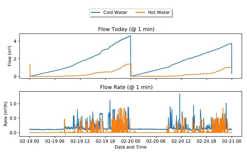
Data 2021, 6, 26                                                                                            2 of 10

                   Relation to Prior Datasets
                         Having received considerable attention from the research community, particularly in
                   recent years, there has also been an effort to release water consumption datasets. In [15],
                   Di Mauroet et al. [15] review 92 urban water demand datasets. The reviewed datasets
                   were distributed across three spatial scales, district (20 datasets), household (31), and
                   end-use (41). Unfortunately, many of these datasets are not available with an open-source
                   license. Instead, some have restricted access (e.g., requiring a commercial license of special
                   requests to the data owners), whereas for others (primarily in papers published in the
                   1970s/80s/90s), there is no information on accessing them.
                         Interestingly, there are no references to water demand in restaurants. Furthermore,
                   a search on data.world (see https://data.world/search (accessed on 1 March 2021)) and
                   openei.org (see https://openei.org/ (accessed on 1 March 2021)) for the keywords “kitchen
                   water” and “restaurant water” did not reveal any relevant results that suggested the
                   existence of such datasets.
                         To the best of our knowledge, FIKWater is one of the few publicly available datasets
                   with water demand from restaurant kitchens. Hence, making this a valuable and unique
                   contribution to the water monitoring and management research fields. More particu-
                   larly, this dataset can be used to develop methodologies to explore water consumption in
                   restaurants [7]. Likewise, this FIKWater can also be used to develop and evaluate water
                   consumption benchmarks across kitchens, which is a topic currently underexplored in
                   the context of electricity consumption (e.g., [16,17]) but not covered when it comes to
                   water demand.
                         From a more technical perspective, FIKWater can also be used in the context of
                   machine-learning research. For example, in the context of non-intrusive water disaggrega-
                   tion [3,5], which identifies the water consumption of individual wet-appliances taking only
                   aggregated water demand measurements. In this context, the fact that FIKWater contains
                   information about individual wet-appliances in one of the kitchens makes it particularly
                   relevant. Finally, this dataset can also serve to further the research in the simulation of wa-
                   ter demand profiles in industrial contexts, which unlike the domestic sector (e.g., [18,19]),
                   is still relatively under-explored, e.g., [20].

                   2. Methods
                        This section provides an overview of the data collection process that leads to creating
                   the FIKWater dataset.

                   2.1. Data Collection Hardware
                        The water consumption was measured using an ultrasonic flow meter, specifically
                   the TUF2000M (see http://www.t3-1.com/english/index.php (accessed on 1 March 2021))
                   installed on the main water entrance pipe, hence monitoring the total water demand. The
                   TUF2000M measures the following parameters: (1) instantaneous flow rate, (2) liquid
                   velocity, (3) speed of sound, (4) positive and negative accumulators, and (5) totals (day,
                   month and year).
                        The main reason to select an ultrasonic flow meter is the fact that they enable monitor-
                   ing the water flow from outside the pipes with clamp-on sensors, hence avoiding invasive
                   changes to the existing infrastructure. Figure 1 shows the used sensor and an illustration
                   of the installation procedure. Table 1 lists the most relevant features of the TUF2000M
                   ultrasonic flow meter.
                        After installing the sensors, it was necessary to set the following parameters in the
                   meter: (1) type of liquid to monitor, (2) internal and external diameter of the pipe, (3)
                   pipe thickness, (4) pipe material, (5) connection type, and (6) distance between the ultra-
                   sonic transducers.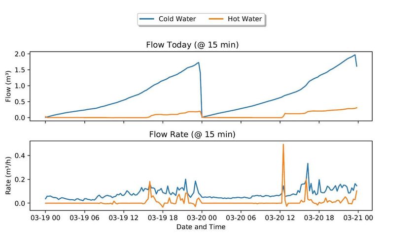
Data 2021, 6, 26                                                                                                     3 of 10

                   Figure 1. Left: TUF2000M Ultrasonic flow meter; Right: illustration of installation.

                    Table 1. Main parameter of the TUF2000M ultrasonic flow meter.

 Parameter         Value
 Accuracy          ≤1%
 Velocity Range    0 ~±10 m/s, bi-directional
 Pipe Size         DN32 DN6000 mm
 Pipe Material     Steel, stainless steel, cast iron, copper, PVC, aluminum, etc.
 Type of Liquid    Single liquid that can transmit ultrasound, such as water, sea water, and oil
 Temperature       ~30 ºC ~160 ºC

                   2.2. Monitoring Platform
                        In order to proceed with the data collection, a bespoke monitoring platform was
                   developed. Figure 2 illustrates the main components of the platform. The clamp-on sensors
                   are placed on the water pipe, measuring the water flow. The monitored data were then sent
                   to the local gateway using the Modbus protocol (see https://modbus.org/ (accessed on 1
                   March 2021)) protocol. The data were stored locally before being uploaded to the Internet
                   using the standard HTTPS protocol.

                                                                            Every Minute

                                         Modbus                  HTTPS                     Database (JSON)

                              Water Flow                                    Everyday at 12AM
                           Clamp-on Sensor             Gateway

                                                                                               Shared Folder (CSV)

                                        Local Area Network                                     Internet

                   Figure 2. Main components of the water consumption monitoring platform (icons by draw.io
                   (accessed on 25 January 2021) and flaticon.com (accessed on 25 January 2021)).

                        Figure 3 shows the block diagram with the gateway’s different components. In
                   simple terms, the system worked as follows. The data acquisition software running in
                   the Raspberry Pi (see https://www.raspberrypi.org/ (accessed on 25 January 2021)) took
                   measurements from the ultrasonic flow meter at predefined S seconds intervals. By default,
                   the value of M was set to five seconds, but it could also be given as an input to the data
                   acquisition algorithm.
                        The collected measurements were stored on a local database. Every minute, the most
                   up-to-date measurements were uploaded to an online database server for providing near
                   real-time data access to interested third-parties (e.g., an application developer). Further-
                   more, every day at 12:00 a.m., a Comma Separated Values (CSV) file with the daily readings
                   was uploaded to a shared folder. Upon successful upload, existing records were deleted
                   from the local database to keep its footprint as light as possible at all times.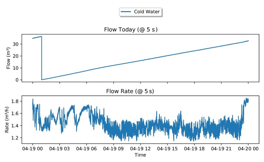
Data 2021, 6, 26                                                                                                 4 of 10

                        A Real Time Clock (RTC) was used to keep track of the time in the gateway and
                   provide timestamps to collected measurements. Finally, a 3S lithium battery was used to
                   allow deployments in places without a power connection and to avoid data losses in case
                   of a power outage since the used sensing device did not have internal memory to store
                   instantaneous measurements.

                   Figure 3. Block diagram showing the different components of the gateway.

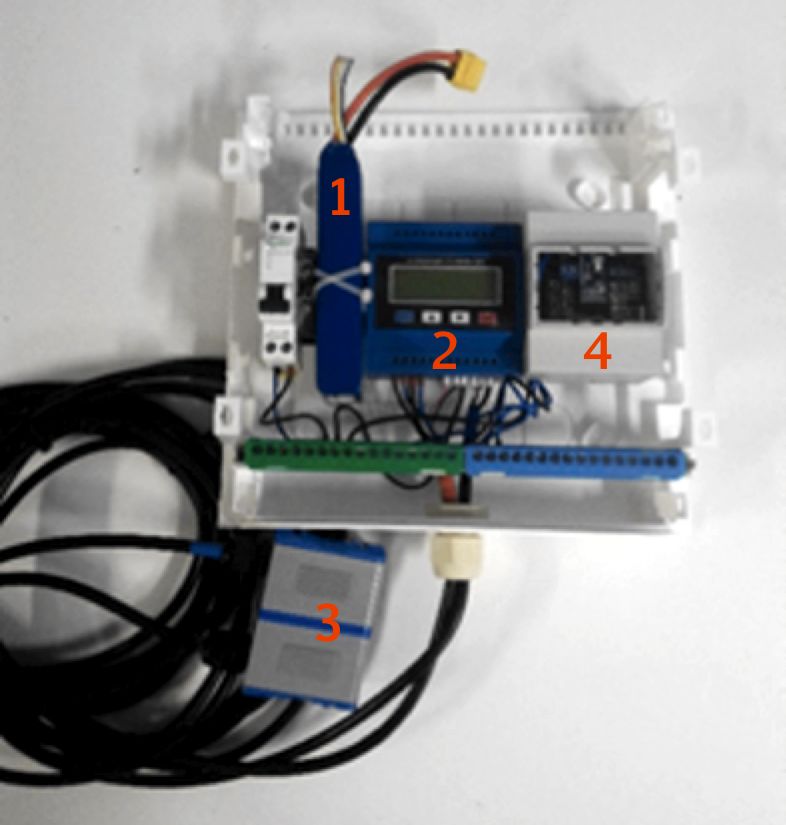
                        Figure 4 shows a picture of the developed prototype, depicting the main components:
                   (1) 3S battery, (2) TUF2000M, (3) Transducers, and (4) Raspberry Pi.

                   Figure 4. Box deployed with all the hardware needed for the water monitoring: (1) 3S battery, (2)
                   TUF2000M, (3) Transducers, and (4) Raspberry Pi.

                   2.3. Deployments
                        The monitoring platform was deployed in three restaurant kitchens for consecutive
                   periods between two (kitchen 1) and four weeks (kitchens 2 and 3). Table 2 summarizes
                   the details of each kitchen.

                   Table 2. Details of the three deployments. The column S refers to the sampling interval

                    ID    Service                 Area (m2 )    Capacity (Seats)        Start          End          S
                     1    Dinner                     58.15              50           15-02-2019     03-03-2019      5
                     2    Dinner                     25.52              50           12-03-2019     02-04-2019      5
                     3    Breakf. and Dinner         35.23              40           16-04-2019     15-05-2019      5

                        In order to monitor both hot and cold water consumption, two monitoring systems
                   were deployed in each kitchen. Figure 5 depicts two of the three deployments of the
                   platforms. Unfortunately, due to physical constraints with the hot water installation of
                   kitchen number 3, the recorded data were not accurate. Therefore it was not possible to
                   add them to the FIKWater dataset.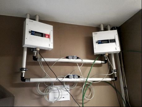
Data 2021, 6, 26                                                                                                 5 of 10

                   Figure 5. The cold and hot water monitoring systems deployed in two of the three monitored kitchens.

                   2.4. Data Labeling
                        To enrich the dataset’s potential applications, FIKWater also contained annotations
                   of the periods when wet appliances (dishwasher and glasswasher) were turned ON or
                   OFF. The annotations were obtained by manually inspecting those appliances’ electricity
                   consumption profiles when such data were available. More precisely, a wet appliance was
                   considered ON when consuming energy for more than 15 consecutive minutes. Conversely,
                   it was considered OFF when there was no consumption, or the observed consumption
                   happened for less than 15 min. The threshold of 15 min was set empirically after observing
                   the electricity consumption of the wet-appliances for the dataset’s duration.

                   3. Data Description
                        The FIKWater dataset was made available individually for each monitored kitchen,
                   and all the data files were in CSV format. Figure 6 shows an overview of the underlying
                   organization of the FIKWater dataset. The following subsections describe the contents of
                   the different files.

                     /
                         data
                            deployments.csv                                    Kitchen 2
                            Kitchen 1                                             demand
                               demand                                                hot_water_demand.csv
                                  hot_water_demand.csv                               cold_water_demand.csv
                                  cold_water_demand.csv                        Kitchen 3
                               labels                                             measurements
                                  dishwasher_labels.csv                              cold_water.csv
                                  glasswasher_labels.csv
                                  wet_appliances.txt

                   Figure 6. Underlying folder and file organization of FIKWater Dataset.

                   3.1. Demand Data
                        The water demand files (_demand.csv) contained the measurements taken from
                   the water flow sensors. These measurements were provided in raw form, i.e., as measured
                   by the sensors. The underlying fields of the measurements files are described in Table 3.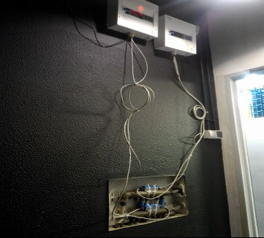
Data 2021, 6, 26                                                                                                     6 of 10

                    Table 3. Column descriptions for the water demand files (_demand.csv).

 Column            Description                                                                            Units
 timestamp         The timestamp when the record was collected                                             –
 flow_rate         Water flow rate                                                                        m3 /h
 velocity          Water velocity                                                                         m/s
 sound_speed       Sound speed in the water                                                               m/s
 flow_today        Total water flow from 00:00 up to this moment                                           m3
 flow_month        Total water flow from the beginning of the month up to this moment                      m3

                        3.2. Labels Data
                             The label files (_labels.csv) identified the periods when wet appliances were
                        turned ON or OFF. The underlying fields are described in Table 4. The technical details of
                        the wet appliances are provided in the wet_appliances.txt file.

                        Table 4. Column descriptions for the label files (_labels.csv).

                          Column               Description                                                 Units
                          timestamp            The timestamp when the label was recorded                     –
                          mode                 If the appliance is ON (0) or OFF (1)                      binary

                        3.3. Deployments
                             The deployments file (deployments.csv) contained additional details of each deploy-
                        ment. The underlying fields are described in Table 5. Note that the Start and End dates
                        refer to the date of the first and last water consumption measurements in each kitchen,
                        respectively. These dates did not necessarily correspond to the start and end dates in
                        Table 2 since these corresponded to the start and end of the FIK monitoring campaigns.

                        Table 5. Column descriptions for the ground truth files (deployments.csv).

                          Column               Description                                                      Units
                          ID                   Kitchen identifier                                             number
                          service              Type of service provided (Breakfast, Lunch, Dinner)              text
                          area                 Area of the kitchen floor                                         m2
                          capacity             Maximum number of customers in simultaneous                    number
                          has_hot_water        If hot water data are available or not                          binary
                          has_cold_water       If cold water data are available or not                         binary
                          has_labels           If the data contain wet appliance labels or not                 binary
                          start                Date of the first measurement across all the waste bins        datetime
                          end                  Date of the last measurement across all the waste bins         datetime

                        4. Data Exploration and Conclusions
                             The number of monitoring days and records collected in the three kitchens are pre-
                        sented in Table 6. Coverage indicates the ratio between the monitored and the expected
                        number of samples at the rate of one sample every five seconds ( 15 Hz), which, as can be
                        observed, was very high across the three kitchens.

                        Table 6. Number of monitoring days and total records in each of the monitored kitchens. The
                        heatmap from blue to read indicates the data availability (dark blue—more data; dark red—less data)

                          ID          Days           Hot Water            Cold Water             Coverage (%)
                           1           18             289,541              289,851                    98
                           2           25             396,936              393,678                    95
                           3           31                –                 522,107                    98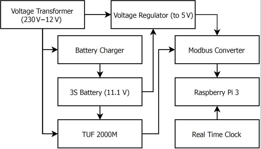
Data 2021, 6, 26                                                                                                                                           7 of 10

                                                            Figure 7 shows the distribution of the daily water flows (flow_today) in each of the
                                                       monitored kitchens. As it can be observed from the water flows in kitchens 1 and 2, cold
                                                       water consumption was much higher than that of hot water. This, in part, happened
                                                       because most of the activities, like cooking and cleaning (normally happening at the end of
                                                       the day), used cold water. On the other hand, hot water was used mostly for dishwashing.
                                                            Furthermore, it was possible to see that the consumption of cold water in kitchen 3
                                                       was much higher than that of the other kitchens (nine times higher than kitchen 1 and 19
                                                       times higher than kitchen 2). After consultation with the kitchen maintenance services,
                                                       it was found that the monitored pipes were not fully dedicated to the kitchen operations.
                                                       As such, a big part of these measurements referred to the consumption of other hotel
                                                       divisions. This effect was also observable in Figure 8 (bottom), which shows that water
                                                       was continuously used over the 24 h.

                                    Kitchen 1                                                  Kitchen 2                                    Kitchen 3
            2.5                                                              2.5                                                       40
                                                                                                                                       35
            2.0                                                              2.0
                                                                                                                                       30
            1.5                                                              1.5                                                       25

                                                                                                                           Flow (m³)
Flow (m³)

                                                                 Flow (m³)

                                                                                                                                       20
            1.0                                                              1.0                                                       15
                                                                                                                                       10
            0.5                                                              0.5
                                                                                                                                       5
            0.0                                                              0.0                                                       0
                        Hot Water                  Cold Water                      Hot Water                  Cold Water                     Cold Water
                                    Water Sensor                                               Water Sensor                                 Water Sensor

                  Figure 7. Boxplots illustrating the distribution of the daily flows of water. Left: kitchen 1, Center: kitchen 2, Right: kitchen 3.
                  The circles represent the smallest and highest outliers found in the data.

                                                       Figure 8. Evolution of the water consumption in kitchen 3 over 24 hours. Top: flow_today; Bottom:
                                                       flow_rate. Note that this data is plotted at the original sampling rate of 15 Hz.

                                                              This clearly contrasts the measurements from kitchens 1 and 2 (see Figure 9), where
                                                       it is evident that water was mostly used during specific periods of the day. For example,
                                                       in kitchen 1, both hot and cold water were used more intensively after 10:00 PM, which
                                                       corresponded to the dinner service’s end.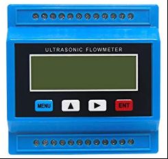
Data 2021, 6, 26                                                                                                                                      8 of 10

      Figure 9. Evolution of the water consumption over 48 h. Left: kitchen 1; Right: kitchen 2. Note that the data are plotted at
                                        1                       1
      different sampling rates, namely 60 Hz in kitchen 1, and 300 Hz in kitchen 2.

                                                        Finally, Figure 10 illustrates the total (hot + cold water) flow rate measurements
                                                   supplemented with the labeled wet appliances transitions. The green dashed line represents
                                                   ON transitions, whereas the red dotted lines represent the OFF events. As can be observed,
                                                   there was also water consumption outside the periods where these appliances were ON,
                                                   representing water uses for other purposes (e.g., cooking or cleaning) or wet appliances
                                                   that were not monitored.

                                                          Flow Rate (Hot + Cold Water)        Wet Appliance ON     Wet Appliance OFF

                                                                                         Dishwasher
                                 1.00
                                 0.75
                   Rate (m³/h)

                                 0.50
                                 0.25
                                 0.00

                                                                                         Glass Washer
                                 1.00
                                 0.75
                   Rate (m³/h)

                                 0.50
                                 0.25
                                 0.00
                                        02-19 00   02-19 06    02-19 12      02-19 18      02-20 00    02-20 06   02-20 12     02-20 18   02-21 00
                                                                                         Date and Time

      Figure 10. Total flow rate (hot + cold water) measurements supplemented with wet appliances transitions (kitchen 1, from
                                                                                                     1
      19 February 2019 to 20 February 2019). Note that this data is plotted at the sampling rate of 300 Hz.

                                                   Author Contributions: conceptualization, L.P. and V.A.; methodology, L.P. and V.A.; software,
                                                   L.P., V.A. and F.V.; validation, L.P., V.A. and F.V.; resources, L.P.; data curation, L.P., V.A. and F.V.;
                                                   writing—original draft preparation, L.P.; writing—review and editing, L.P. and V.A.; visualization,
                                                   L.P.; supervision, L.P.; project administration, L.P.; funding acquisition, L.P. All authors have read
                                                   and agreed to the published version of the manuscript.
                                                   Funding: This research was funded by project M1420-01-0247-FEDER-000018 (Madeira 14-20). Lucas
                                                   Pereira received funding from the Portuguese Foundation for Science and Technology (FCT) under
                                                   grants CEECIND/01179/2017 and UIDB/50009/2020.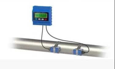
Data 2021, 6, 26                                                                                                                       9 of 10

                                   Data Availability Statement: The data presented in this study are openly available in Open Science
                                   Framework (OSF) at doi 10.17605/OSF.IO/7BZ2M, reference number 7bz2m.
                                   Acknowledgments: We would like to acknowledge all the staff in the monitored kitchens and the
                                   technicians that assisted in planing and performing the three deployments of the monitoring platform.
                                   Conflicts of Interest: The authors declare no conflict of interest.

                                   Abbreviations
                                   The following abbreviations are used in this manuscript:

                                   CSV Comma Separated Values
                                   FIK Future Industrial Kitchen
                                   IK Industrial Kitchen
                                   IoT Internet of Things
                                   OSF Open Science Framework
                                   RTC Real Time Clock

References
1.    Froehlich, J.E.; Larson, E.; Campbell, T.; Haggerty, C.; Fogarty, J.; Patel, S.N. HydroSense: Infrastructure-mediated single-point
      sensing of whole-home water activity. In Proceedings of the 11th International Conference on Ubiquitous Computing, UbiComp
      ’09, Orlando, FL, USA, 30 September–3 October 2009; Association for Computing Machinery: New York, NY, USA, 2009;
       doi:10.1145/1620545.1620581.
2.    Richter, C.P.; Stamminger, R. Water Consumption in the Kitchen—A Case Study in Four European Countries. Water Resour.
      Manag. 2012, 26, 1639–1649. doi:10.1007/s11269-012-9976-5.
3.    Ellert, B.; Makonin, S.; Popowich, F. Appliance Water Disaggregation via Non-intrusive Load Monitoring (NILM). In Smart City
      360◦ ; Leon-Garcia, A., Lenort, R., Holman, D., Staš, D., Krutilova, V., Wicher, P., Cagáňová, D., Špirková, D., Golej, J., Nguyen, K.,
      Eds.; Lecture Notes of the Institute for Computer Sciences, Social Informatics and Telecommunications Engineering; Springer
      International Publishing: Cham, Switzerland, 2016; pp. 455–467.
4.    Hussien, W.A.; Memon, F.A.; Savic, D.A. An integrated model to evaluate water-energy-food nexus at a household scale. Environ.
      Model. Softw. 2017, 93, 366–380. doi:10/gfrd5k.
5.    Pastor-Jabaloyes, L.; Arregui, F.J.; Cobacho, R. Water End Use Disaggregation Based on Soft Computing Techniques. Water 2018,
      10, 46. doi:10/gc8mf9.
6.    Murakawa, S.; Takata, H.; Nishina, D. Development of the Calculating Method for the Loads of Water Consumption in Restaurant.
      In Proceedings of the 30th W062 International Symposium on Water Supply and Drainage for Buildings, Paris, France, 16–17
      September 2004; p. 14.
7.    Murakawa, S.; Nishina, D.; Takata, H.; Tanaka, A. An Analysis on the Loads of Hot Water Consumption in the Restaurants. In
      Proceedings of the 31st W062 International Symposium on Water Supply and Drainage for Buildings, Brussels, Belgium, 14–16
      September 2005; p. 11.
8.    Delagah, A.; Davis, R.; Slater, M.; Karas, A. Results from 20 Field Monitoring Projects on Rack and Flight Conveyor Dishwashers
      in Commercial Kitchens. ASHRAE Trans. 2007, 123. Available online: https://go.gale.com/ps/anonymous?id=GALE%7CA490
      983843&sid=googleScholar&v=2.1&it=r&linkaccess=fulltext&issn=00012505&p=AONE&sw=w (accessed on 1 March 2021).
9.    Deng, S. Energy and water uses and their performance explanatory indicators in hotels in Hong Kong. Energy Build. 2003,
      35, 775–784. doi:10.1016/S0378-7788(02)00238-4.
10.   Alonso, A.D. How Australian Hospitality Operations View Water Consumption and Water Conservation: An Exploratory Study.
      J. Hosp. Leis. Mark. 2008, 17. doi:10.1080/10507050801984917.
11.   Angulo, A.; Atwi, M.; Barberán, R.; Mur, J. Economic Analysis of the Water Demand in the Hotels and Restaurants Sector:
      Shadow Prices and Elasticities. Water Resour. Res. 2014, 50, 6577–6591. doi:10.1002/2013WR014085.
12.   Gabarda-Mallorquí, A.; Garcia, X.; Ribas, A. Mass tourism and water efficiency in the hotel industry: A case study. Int. J. Hosp.
      Manag. 2017, 61, 82–93. doi:10.1016/j.ijhm.2016.11.006.
13.   Pereira, L.; Aguiar, V.; Vasconcelos, F. Future Industrial Kitchen: Challenges and Opportunities. In Proceedings of the 6th ACM
      International Conference on Systems for Energy-Efficient Buildings, Cities, and Transportation, BuildSys ’19, New York, NY, USA,
      13–14 November 2019; ACM: New York, NY, USA, 2019; pp. 163–164. doi:10/ggfhm7.
14.   Vasconcelos, F.; Aguiar, V.; Pereira, L. Ultrasonic waste monitoring in the future industrial kitchen: poster abstract. In Proceedings
      of the 17th Conference on Embedded Networked Sensor Systems, SenSys ’19, New York, NY, USA, 10–13 November 2019;
      Association for Computing Machinery: New York, NY, USA, 2019; pp. 446–447. doi:10.1145/3356250.3361960.
Data 2021, 6, 26 10 of 10
15. Di Mauro, A.; Cominola, A.; Castelletti, A.; Di Nardo, A. Urban Water Consumption at Multiple Spatial and Temporal Scales. A
Review of Existing Datasets. Water 2021, 13, 36. doi:10.3390/w13010036.
16. Hedrick, R.; Smith, V.; Field, K. Restaurant Energy Use Benchmarking Guideline; Technical Report NREL/SR-5500-50547, 1019165;
NREL: Golden, CO, USA, 2018. doi:10.2172/1019165.
17. Mudie, S. Energy Benchmarking in UK Commercial Kitchens. Build. Serv. Eng. Res. Technol. 2016, 37, 205–219. doi:10/f8d998.
18. Zaher, R.; Chaccour, K.; Badr, G. Intelligent Software Simulation of Water Consumption in Domestic Homes. In Proceedings of
the 2016 UKSim-AMSS 18th International Conference on Computer Modelling and Simulation (UKSim), Cambridge, UK, 6–8
April 2016; pp. 99–104. doi:10.1109/UKSim.2016.30.
19. Ritchie, M.J.; Engelbrecht, J.A.A.; Booysen, M.J. A Probabilistic Hot Water Usage Model and Simulator for Use in Residential
Energy Management. Energy Build. 2021, 235, 110727. doi:10.1016/j.enbuild.2021.110727.
20. Blokker, E.J.M.; Pieterse-Quirijns, E.J.; Vreeburg, J.H.G.; van Dijk, J.C. Simulating Nonresidential Water Demand with a Stochastic
End-Use Model. J. Water Resour. Plan. Manag. 2011, 137, 511–520. doi:10.1061/(ASCE)WR.1943-5452.0000146.You can also read


