Time Tagged Time-Resolved Fluorescence Data Collection in Life Sciences
←
→
Page content transcription
If your browser does not render page correctly, please read the page content below
Technical Note
Time Tagged Time-Resolved Fluorescence Data Collection in
Life Sciences
Michael Wahl, Sandra Orthaus-Müller
PicoQuant GmbH, Rudower Chaussee 29, 12489 Berlin, Germany, info@picoquant.com
Motivation processes can be observed independently from the
fast dynamics related to fluorescence lifetime, and
Fluorescence lifetime measurements in the time even with CW illumination, the related techniques
domain are commonly performed by means of and instruments have until recently evolved rather
Time-Correlated Single Photon Counting (TCSPC). independently. If both phenomena were of interest,
Classical TCSPC is a histogramming technique researchers would usually conduct independent ex-
based on precise timing and time binned counting of periments. However, given the ‘transient’ nature of
single photons emitted on pulsed laser excitation[1],[2]. many single molecule experiments (consider, e.g.,
However, in many fluorescence applications it is of photobleaching), it turned out to be of great value to
great interest not only to obtain the fluorescence life- be able to link effects on both time scales in one ex-
time(s) of the fluorophore(s) but to record and use periment. For instance, in capillary flow experiments,
more information on the fluorescence dynamics. the millisecond dynamics can help to identify a sin-
This is most often the case when very few or even gle molecule transit, while the picosecond to nano-
single molecules are observed. For instance, in Fluo- second dynamics (e.g., fluorescence lifetime) can
rescence Correlation Spectroscopy (FCS), the infor- be used to distinguish different species. This can be
mation of interest is contained in the intensity fluctua- achieved by using a pulsed excitation source (e.g.,
tions caused by the diffusion of fluorescent molecules picosecond pulsed laser), and a fluorescence detec-
through a small detection volume. These diffusion tion set-up that allows for picosecond time resolution
related fluctuations occur on a millisecond time scale with respect to the excitation pulses.
and are typically analyzed by means of an autocor- In addition, the capability of intensity recording
relation of the fluctuation signal. This gives access with sub-millisecond resolution must be ensured.
to concentrations and diffusion constants and there- The recording of the fast dynamics (fluorescence
by to molecule mobility and/or size. Similarly, single decay) is commonly implemented via TCSPC. The
molecules flushed through capillaries (e.g in DNA arrival times recorded in the TCSPC histogram are
analysis applications) will emit short bursts of fluo- relative times between a laser excitation pulse and
rescence, that are of interest for further analysis. The the corresponding fluorescence photon arrival times
resulting fluorescence intensity dynamics on a time at the detector. These measurements are ideally re-
scale of milliseconds can be used to identify single solved down to a few picoseconds. After collection of
molecule transits and to discriminate these events sufficient photon numbers, one or more fluorescence
against background noise. Even with immobilized lifetimes can be calculated.
single molecules, characteristic blinking behavior of TCSPC can be implemented with a variety of in-
continuously excited molecules can be observed, strumentation, but not many designs are suitable to
again on a millisecond time scale. The analysis record the slower intensity dynamics at the same
and interpretation of the underlying processes has time. This is because the intensity dynamics infor-
become a research topic in its own. Since all these mation is not available from conventional histograms
1from TCSPC data, often collected over minutes. To cal TCSPC timing covers the picosecond time scale
solve the problem one can continuously collect histo- between laser pulses, the additional time tags allow
grams over very short intervals. This direct approach covering the whole time range of seconds, minutes
was successful in early capillary flow experiments, or even hours, thereby providing ultimate flexibility in
but is hampered by data acquisition bottle necks, further data analysis. The two timing figures (TCSPC
since it generates large amounts of redundant data. time and time tag) are stored as one photon record. If
This is because at the (necessary) short time slices the TCSPC device has more than one detector chan-
per histogram, the histograms are mostly empty. Still nel (either natively[7],[8] or by means of a router[6]) then
they must be fully processed and stored. Even if the the channel code is also stored in the photon record
histogramming is performed in integrated hardware, (Figure 2).
e.g., on PC boards with dedicated memory, the re- In order to work efficiently with current host com-
dundant data processing is not very elegant and lim- puters, the photon record is typically chosen as a 32
its remain due to on-board memory constraints. bit structure. Current TTTR hardware designs are
Furthermore, it is often desirable to have as much implemented in Field Programmable Gate Arrays
information as possible about all photon events for (FPGA). A large First In First Out (FIFO) buffer is
further analysis. Even histogramming with very fast used to average out bursts and deliver a moderate
time slices would reduce the original information con- constant data rate to the host interface. This way suf-
tent. It is therefore far more elegant to record each ficient continuous sustained transfer rates are pos-
fluorescence photon as a separate event, and to sible in real-time, even when photon rates are high.
consider fluorescence lifetime histogramming as one Most recent devices use PCI express or USB 3.0
out of many analysis methods that can be applied to where continuous transfer rates as high as 40 Mcps
the photon stream, be it on-line or off-line. can be handled[7],[8].
Basic Concept TTTR with Multiple Detectors and
Marker Signals
The desired capturing of the complete fluorescence
dynamics can be achieved by recording the arrival Fluorescence Lifetime Imaging (FLIM), which is a
times of all photons relative to the beginning of the powerful extension to fluorescence imaging micros-
experiment (time tag), in addition to the picosec- copy. In order to perform FLIM, the spatial origin
ond TCSPC timing relative to the excitation pulses. of the photons must be recorded in addition to the
This is called Time-Tagged Time-Resolved (TTTR) TCSPC data. Conventional systems use a large ar-
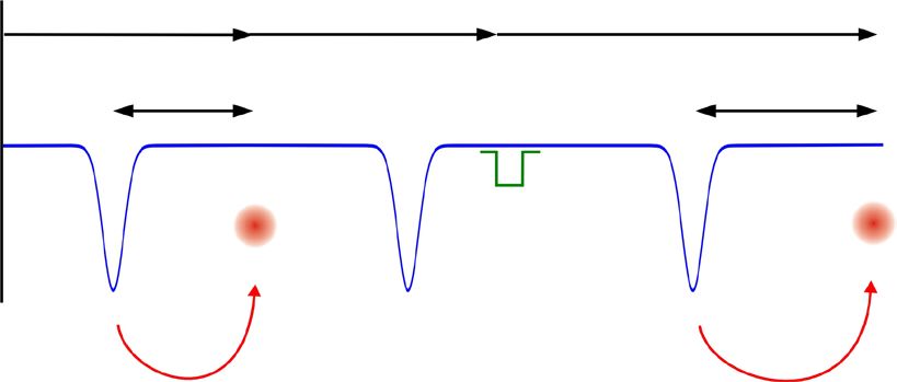
mode[2]. Figure 1 shows the relationship of the time rays of on-board memory to accommodate the large
figures involved. amount of data generated due to the multidimension-
As in conventional TCSPC, a picosecond timing al matrix of pixel coordinates and lifetime histogram
between laser pulse and fluorescence photon is ob- channels. Even with modern memory chips, this
tained. In addition to that, in TTTR data collection approach still used in some competing products is
a coarser timing is performed on each photon with very limited in image size. Consequently, it is expen-
respect to the start of the experiment. This is done sive, and implies loss of information. Furthermore,
with a digital counter running typically at 50 or 100 ns the time per pixel is usually limited. Still, in order to
resolution. Most recent devices actually use the ex- obtain lifetime information, a TCSPC histogram must
citation pulses for this counter[6],[7],[8]. Since the classi- be formed for each pixel. This makes it difficult to
Figure 1: Timing figures in TTTR data acquisition.
2Figure 2: TTTR data acquisition scheme with routing and external markers.
construct suitable hardware at reasonable cost. To markers was copied by competitors.
solve the problem much more elegantly, the TTTR As outlined briefly above, PicoQuant’s TTTR
data stream can be extended to contain markers for hardware is designed to include channel information
synchronization information derived from an imag- for multiple detectors. In case of the PicoHarp 300,
ing device, e.g., a piezo scanner. This makes pos- four detector channels can be provided by means
sible to reconstruct the 3D image from the stream of a router[6]. This is a cost efficient solution but can
of TTTR records, since the relevant XYZ position have limitations in correlation experiments across
of the scanner can be determined during the data channels. In case of the HydraHarp 400 and the
analysis. The data generated is free of redundancy TimeHarp 260 there are truly independent detector
and can therefore be transferred in real-time, even if channels natively provided[7],[8]. From the perspective
the scan speed is very fast, like, e.g., in Laser Scan- of TTTR mode it does not matter if the channel infor-
ning Microscopes (LSM). The image size is unlimited mation comes from independent timing circuits. A nu-
both in XYZ and in count depth. Since there are up to merical channel code is recorded in the data stream
four such synchronization signals, all imaging appli- and can be recovered later. Having multiple detector
cations can be implemented and even other exper- channels available, one can record, e.g., different
iment control signals can be recorded. This marker emission wavelengths or multiple polarization states
scheme is a very special feature of the PicoQuant in parallel. (Figure 3)
TCSPC electronics[6],[7],[8]. It may be worth noting that Typically, routing and synchronization information
this technology enabled PicoQuant to develop the are fed to the TTTR hardware as TTL signals from
leading edge MicroTime 200 Fluorescence Lifetime the external devices. Figure 2 shows how such addi-
Microscope. Only much later the concept of TTTR tional information is inserted in the TTTR data.
3Figure 3: Multichannel TCSPC.
In an imaging application the external markers from TTTR data by evaluating only the time tags of
signals are typically connected such that they cor- the photon records. Sequentially stepping through
respond to ‘start of line’ or ‘start of pixel’ in an image the arrival times, all photons within the chosen time
scan. Sequentially stepping through the data records bins (typically milliseconds) are counted. This gives
it is then straight forward to form TCSPC histograms access to, e.g., single molecule bursts (in flow) or
for all pixels and calculating their fluorescence life- to blinking dynamics. The bursts can be further an-
time(s). These can then be evaluated and color-cod- alyzed, e.g., by histogramming for burst height and
ed according to their intensity as well as lifetime. frequency analysis.
Fluorescence lifetimes can be obtained by histo-
gramming the TCSPC (start-stop) times and fitting
of the resulting histogram, as in the conventional ap-
TTTR Data Analysis and Typical proach. In single molecule applications with very few
counts per histogram, faster algorithms based on
Applications maximum likelihood criteria are used. When the ob-
jective is mere distinction of multiple species with a
Time-Tagged Time-Resolved (TTTR) measurement priori known fluorescence lifetimes, even simpler and
mode allows to perform vastly different measurement more speed efficient algorithms can be employed.
tasks based on one single data format, yet without The strength of the TTTR format is best exploit-
any sacrifice of information available from each sin- ed when both time figures are used together. For in-
gle photon. This in turn allows to handle all measure- stance, one can first evaluate the MCS trace to iden-
ment data in a standardized and yet flexible way. The tify single molecule bursts, and then use the TCSPC
concept is without redundancy in the data stream, times within those bursts, to evaluate fluorescence
but also without any loss of information, as opposed lifetimes for individual bursts (Figure 5). If there
to, e.g., in onboard histogramming. Therefore, virtu- are different molecular species with different fluo-
ally all algorithms and methods for the analysis of rescence lifetimes, this can be used to distinguish
fluorescence dynamics, such as intensity time trace them in real-time, e.g., in capillary flow approaches
analysis, burst analysis, lifetime histogramming, to DNA sequencing or substance screening. Vice
Fluorescence Correlation Spectroscopy (FCS), and versa, one can employ time gating on the TCSPC
Fluorescence Lifetime Imaging (FLIM) can be imple- time before evaluating the intensity trace, i.e., one
mented. Figure 4 shows a summary of the methods rejects all photons that do not fall in a time span that
that can be applied by using TTTR data. is likely to contain fluorescence photons. This time
Intensity traces over time, as traditionally obtained gating reduces noise from background and scattered
from Multi-Channel-Scalers (MCS), are obtained excitation light.
4Figure 4: Data display and analysis methods applicable with TTTR data.
A powerful application of TTTR mode and time
gating is FCS. Traditionally, FCS was performed by
hardware correlators, because the computational de-
mand of the correlation function is considerable, and
results are often desired to be available in real-time.
However, hardware correlators have some disadvan-
tages. One is that they usually do not calculate the
correlation function in the strict mathematical sense.
This is because simplifications such as coarser bin-
ning towards longer lag times and data quantization
(rounding) are employed in order to reduce the com-
putation load and memory requirements. The other
is that they perform an immediate (real-time) data
reduction, that does not allow to recover the original
data, and that prohibits to ‘slice’ the data if parts of
it turn out to be unusable during the measurement.
This is the case, e.g., in diffusion experiments, when
large undesired particles enter the focal volume. The
scatter or strong fluorescence from these particles
will then immediately enter the previously collected
correlation function and ‘swamp’ it irreversibly with Figure 5: Single molecule lifetime variations over time evaluated
artifacts. Having individual photon records available by using TTTR. (A) Time trace and (B) fluorescence lifetime his-
togram of single Cy5 molecules, acquired with a MicroTime 200
from TTTR mode, one can perform the correlation using pulsed 635 nm excitation. The lifetime of the two selected
in software and select the ‘good’ data, or data of in- molecules (green and red region in MCS trace and decay) and
terest, as required. On modern computers and with was fitted to 1.6 ns and 0.65 ns, respectively.
5recently developed fast algorithms it is possible to aging with the TTTR approach. Important examples
perform the correlation even in real-time[3]. Further- include Förster Resonance Energy Transfer (FRET)
more, off-line analysis can be repeated infinitely and fluorescence anisotropy methods (Figure 7).
with variations in the analysis approach, if in-depth Indeed, due to the virtually unlimited choices in
investigations in basic research are desired. Finally, data analysis, TTTR mode is a very powerful key
the ultimate strength in TTTR based FCS analysis to molecular imaging. Because it allows to combine
is again the combination of the two time figures. As fluorescence imaging with, e.g., Multiparameter Flu-
a first useful approach, one can employ time gat- orescence Detection[5] for thorough analysis of fluo-
ing on the TCSPC time to reject scatter and back- rescence dynamics, the method is used in the most
ground noise. More complex algorithms are subject advanced time resolved fluorescence microscopes
of ongoing research. One very powerful algorithm of available today[6]. (Figure 8)
this kind is called Fluorescence Lifetime Correlation
Spectroscopy. It uses TTTR data to implement a life-
time-weighted or ‘filtered’ variant of FCS that allows
to separate different molecular species in a mixture, Distinction of Specialized TTTR Data
in one single FCS measurement[4]. By filtering the
photon events according to their TCSPC time before Acquisition Modes
they enter the correlation, one can obtain the sep-
arated FCS curves of the species (Figure 6). How- The basic concept of TTTR data collection we in-
ever, the mathematical idea behind FLCS is much troduced in the previous sections is what historical-
more general. Indeed the filter concept can also be ly evolved first. In modern instruments today this
used to suppress detector artifacts (afterpulsing) and scheme is referred to as T3 mode. There is actually
background noise. another mode we call T2 mode. In the following we
Yet another elegant application of TTTR mode is describe some more details of these two modes of
in Fluorescence Lifetime Imaging (FLIM), which is a time tagged data collection. Essentially the distinc-
powerful extension to fluorescence imaging micros- tion of the two modes has to do with the role of the
copy. In order to perform FLIM, the spatial origin SYNC input of the TCSPC device, i.e., the timing in-
of the photons must be recorded in addition to the put where typically the laser synchronization pulses
TCSPC data. As outlined above, this is done by feed- are fed in.
ing position marker signals from a scan stage into the Imagine, we had the option of creating a ‘perfect’
TTTR data stream. This permits the reconstruction of instrument that would be able to capture ALL timing
2D or 3D images from the collected photon records. events regardless of what they are, i.e., laser ex-
Once such imaging capability is set up, there are citation events or photon events from different de-
many further methods that can be taken over to im- tectors. If we can capture all these events with the
Figure 6: Simplified principle of FLCS (Fluorescence Lifetime Correlation Spectroscopy).
6Figure 7: Examples for image analysis possibilities based on TTTR data acquisition. (A) Fluorescence intensity image, (B) FLIM image
and (C) Anisotropy image of single Cy5 fluorescent molecules, acquired with a MicroTime 200 using pulsed 635 nm excitation and two
detection channels for parallel and perpendicular polarization.
Figure 8: Multiparameter Fluorescence Detection (MPD) followed by combined FRET and cross-correlation analysis for investigation of
molecular folding dynamics. In this example, the flexible tetraloop and tetraloop receptor were labeled with donor Cy3 and acceptor Cy5,
respectively, to monitor the Mg 2+-driven RNA folding.
7best possible resolution of our TDCs (Time-to-Dig- of the data stream a theoretically infinite time span
ital-Converters) over an unlimited time span then it can be recovered at full resolution. Dead times exist
no longer necessary to distinguish a fine and coarse only within each channel but not across the chan-
timing in the data records. Everything could then be nels. Therefore, cross correlations can be calculated
calculated from the raw event times. This is what down to zero lag time. This allows powerful applica-
T2 mode is about. We will take a closer look at this tions such as coincidence correlation and FCS with
mode now, but we will see that T3 mode is still need- lag times from picoseconds to hours. Autocorrela-
ed in practice. tions can also be calculated at the full resolution but
of course only starting from lag times larger than the
dead time.
The 32 bit event records are queued in a FIFO
T2 Mode (First In First Out) buffer capable of holding sev-
eral millions of event records. The FIFO input is
fast enough to accept records at the full speed of
In T2 mode all timing inputs of the TCSPC device the TDCs. This means, even during a fast burst no
are functionally identical. There is no dedication of events will likely be dropped except those lost in the
the SYNC input channel to a sync signal from a laser dead time. The FIFO output is continuously read by
(Figure 9A). Instead, it can be used for an addition- the host PC, thereby making room for fresh incom-
al detector signal. The events from all channels are ing events. Even if the average read rate of the host
recorded independently and treated equally. In each PC is limited, bursts with much higher rate can be
case an event record is generated that contains in- recorded for some time. Only if the average count
formation about the channel it came from and the rate over a long period of time exceeds the read-
arrival time of the event with respect to the over- out speed of the PC, a FIFO overrun could occur.
all measurement start. The time tags are recorded In case of a FIFO overrun the measurement must
with the highest resolution the hardware supports be aborted because data integrity cannot be main-
(currently 1, 4, or 25 ps for the different PicoQuant tained. However, on a modern and well configured
TCSPC devices)[6],[7],[8]. PC a sustained average count rates of 40 Mcps are
Each T2 mode event record consists of 32 bits. possible with the TimeHarp 260 and HydraHarp 400.
Going by the example of the data format of the This total transfer rate must be shared by the inputs
TimeHarp 260 and HydraHarp 400, there are 6 bits used. For all practically relevant photon detection ap-
for the channel number and 25 bits for the time tag. plications the effective rate per channel is more than
If the time tag overflows, a special overflow record is sufficient.
inserted in the data stream, so that upon processing For maximum throughput, T2 mode data streams
Figure 9: TTTR data acquisition modes. (A) T2 mode. (B) T3 mode.
8are normally written directly to disk, without preview a compatible resolution R, it is possible to reason-
other than count rate and progress display. However, ably accommodate all relevant experiment scenari-
it is also possible to analyze incoming data ‘on the os. R can be chosen in doubling steps of the card’s
fly’. The generic data acquisition software provided base resolution.
at no extra cost includes a basic real-time correla- Dead time in T3 mode is the same as in the oth-
tor for preview during a T2 mode measurement. The er modes (hardware model dependent). Within each
high-end software SymPhoTime 64 offers a similar photon channel, autocorrelations can be calculated
real-time correlator and many more advanced off- meaningfully only starting from lag times larger than
line analysis methods. the dead time. Across channels dead time does not
affect the correlation so that meaningful results can
be obtained at the chosen resolution, all the way
down to zero lag time.
T3 Mode The 32 bit event records are queued in a FIFO
(First In First Out) buffer just like in T2 mode. The
FIFO input is fast enough to accept records at the
In T3 mode the SYNC input is dedicated to a period- full speed of the time-to-digital converters. There-
ic sync signal, typically from a laser (Figure 9B). As fore, even during a fast burst no events will like-
far as the experimental set-up is concerned, this is ly be dropped except those lost in the dead time.
similar to classical TCSPC histogramming. The main The FIFO output is continuously read by the host
objective is to allow high sync rates which could not PC, thereby making room for new incoming events.
be handled in T2 mode due to TDC dead time and Even if the average read rate of the host PC is lim-
bus throughput limits. Accommodating the high sync ited, bursts with much higher rate can be recorded
rates in T3 mode is achieved as follows: First, a sync for some time. Only if the average count rate over a
divider is employed as in histogramming mode. This long period of time exceeds the readout speed of the
reduces the sync rate so that the channel dead time PC, a FIFO overrun could occur. In case of a FIFO
is no longer a problem. The remaining problem is overrun the measurement must be aborted because
now that even with the divider, the sync event rate data integrity cannot be maintained. However, on a
may still be too high for collecting all individual sync modern and well configured PC a sustained average
events like ordinary T2 mode events. Considering count rates of 40 Mcps are possible (TimeHarp 260
that sync events are not of primary interest, the solu- and HydraHarp 400). This total transfer rate must be
tion is to record them only if they arrive in the con- shared if the device has two detector input channels.
text of a photon event on any of the input channels. For all practically relevant photon detection applica-
The event record is then composed of two timing tions it is more than sufficient.
figures: 1) the start-stop timing difference between For maximum throughput, T3 mode data streams
the photon event and the last sync event, and 2) the are normally written directly to disk. However, it is
arrival time of the event pair on the overall experi- also possible to analyze incoming data ‘on the fly’.
ment time scale (the time tag). The latter is obtained One such analysis method (typically used for FCS)
by simply counting sync pulses. From the T3 mode is the on-line correlation implemented in the device’s
event records it is therefore possible to precisely de- native software. Other specialized analysis methods
termine which sync period a photon event belongs are provided by the SymPhoTime 64 software of-
to. Since the sync period is also known precisely, fered by PicoQuant.
this furthermore allows to reconstruct the arrival time
of the photon with respect to the overall experiment
time.
Each T3 mode event record consists of 32 bits.
Going by the example of the data format of the
TimeHarp 260 and HydraHarp 400, there are 6 bits
for the channel number, 15 bits for the start-stop time
and 10 bits for the sync counter. If the counter over-
flows, a special overflow record is inserted in the data
stream, so that upon processing of the data stream
a theoretically infinite time span can be recovered.
The 15 bits for the start-stop time difference cover a
time span of 32,768×R where R is the chosen resolu-
tion. For example, at the highest possible resolution
of the HydraHarp 400 (1 ps) this results in a span
of 32 ns. If the time difference between photon and
the last sync event is larger, the photon event cannot
be recorded. This is the same as in histogramming
mode, where the number of bins is larger but also
finite. However, by choosing a suitable sync rate and
9References and Further Reading
[1] O’Connor, D. V. O.; Phillips, D. (1984) “Time-correlated Single Photon Counting”, Academic Press,
London
[2] Wahl, M. (2014) Technical Note on TCSPC
[3] Wahl, M.; Gregor, I.; Patting, M.; Enderlein, J. (2003) Optics Express, 11, 26, 3586
[4] Böhmer, M.; Wahl, M.; Rahn, H.-J.; Erdmann, R.; Enderlein, J. (2002) Chem. Phys. Lett.,
353, 5-6, 439-445
[5] C. A. M. Seidel, P. J. Rothwell et al., (2003) Proc. Natl. Acad. Sci. USA, 100, 1655
[6] Wahl M., Rahn H.-J., Gregor I., Erdmann R., Enderlein J. (2007) Rev. Sci. Instrum., 78, 033106
[7] Wahl M., Rahn H.-J., Röhlicke T., Kell G., Nettels D., Hillger F., Schuler B., Erdmann R. (2008)
Rev. Sci. Instrum., 79, 123113
[8] Wahl M., Röhlicke T., Rahn H.-J., Erdmann , R., Kell G., Ahlrichs, A., Kernbach, M., Schell,
A. W., Benson, O. (2013) Rev. Sci. Instrum., 84, 043102
PicoQuant GmbH Phone +49-(0)30-6392-6929
Rudower Chaussee 29 (IGZ) Fax +49-(0)30-6392-6561
12489 Berlin Email info@picoquant.com
Germany WWW http://www.picoquant.com
Copyright of this document belongs to PicoQuant GmbH. No parts of it may be reproduced, translated or transferred to third parties
without written permission of PicoQuant GmbH. All Information given here is reliable to our best knowledge. However, no responsibility
is assumed for possible inaccuracies or ommisions. Specifications and external appearances are subject to change without notice.
© PicoQuant GmbH, 2014
10You can also read