A Beginner's Guide to Deep Learning - IBM Community
←
→
Page content transcription
If your browser does not render page correctly, please read the page content below
A Beginner’s Guide to Deep Learning

                                                            This content was prepared for “For Coders
                                                            and Non-Coders: Break into Deep Learning
                                                            with Python and IBM Watson Studio,” a
                                                            session at IBM Think 2021. The session was
                                                            presented by Alex Amari and Cedric Jouan,
                                                            data scientists with IBM Data and AI Expert
                                                            Labs. The following lab guide was prepared
                                                            by Alex Amari (alexamari@ibm.com).

1.1 AI vs. Machine Learning vs. Deep Learning
Let’s begin with a brief talk on the relationship between Artificial Intelligence (AI), Machine Learning,
and Deep Learning. You’re probably already somewhat familiar with AI, but to give it a precise definition,
we’ll paraphrase one developed by two of the leading experts in the field, Peter Norvig and Stuart
Russell. They define AI as the design and building of intelligent agents (computer systems) that take
information from an environment (data) and use it to take actions that affect that environment. AI, on
this view, comprises the panoply of computational methods and applications that both analyze and
transform data.

What about Machine Learning? The term refers to a broad set of computer algorithms (processes or sets
of rules followed in calculations) that form this bridge between the inputs (data) the outputs
(predictions, classifications, etc.) of AI systems. Another more formal definition for Machine Learning:
“The study of computer algorithms that improve automatically through experience and by the use
of data.”1 When people talk about AI,
they’re almost always talking about systems
built using machine learning. Indeed,
advances in machine learning are the main
reasons why we’ve seen such a huge rise in
interest in AI over the past decade or so.

And finally, Deep Learning. Deep learning is
a simply a subset of machine learning that
focuses on a specific kind of computer
algorithm known as the artificial neural
network. The word neural derives from
neuron, the fundamental type of cell in our

1
    Mitchell, Tom (1997). Machine Learning.

© 2021 IBM Corporation                                                                                    1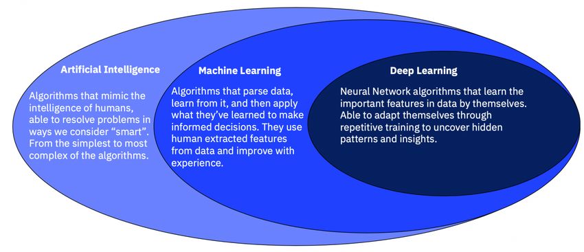
brains. So as the name suggests, these neural networks attempt to simulate the behavior of the human
brain—albeit far from matching its ability—allowing it to “learn” from large amounts of data. Neural
networks can consist of one or multiple layers of “neurons,” and adding more layers tends to increase
the network’s ability to successfully perform whatever task we’re trying to get it to do (such as
classifying images—e.g. is this a picture of a dog or a cat?). When a neural network contains more than
one intermediate “hidden” layer, it is said to be a “deep” neural network. Hence, the term “Deep
Learning.”
We’ll be talking much more about neural networks for the remainder of this lab, but for now you can
think of the relationship between AI, Machine Learning, and Deep Learning in terms of this (crude)
diagram.
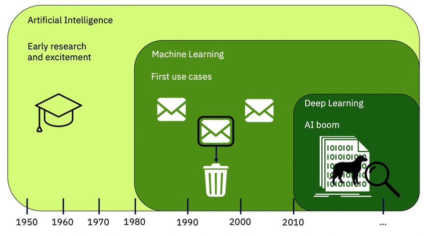
1.2 Why Deep Learning? Pros and Cons
The approaches behind Machine Learning and Deep Learning have actually existed for quite some time.
Around the 1980’s the field of AI began gravitating strongly towards Machine Learning, focusing on what
we now call “Classical” ML
algorithms and approaches.
Similarly, the artificial neural
networks that we use today were
conceived as early as the 1970’s.
However, the field of AI did not
fully embrace Deep Learning until
the early 2010’s—after which
we’ve seen an explosion of Deep
Learning use cases and
applications.
© 2021 IBM Corporation 2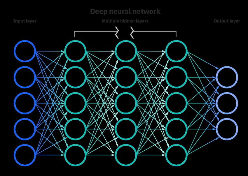
The main reason for this shift is that Deep Learning is computationally expensive—more so than most
classical Machine Learning approaches—and it’s only been in the past decade or so that computers
became powerful enough to make neural networks practical. Today’s neural networks rely on large
amounts of “training data” to work well. More powerful computers mean that more data can be
collected—and ultimately used to train neural networks for tasks like pattern discovery, image
recognition, and content generation.

Deep Learning Pro #1: Performance

Although it is computationally and data-intensive, Deep Learning often outperforms classical Machine
Learning approaches. And there are some tasks that lend themselves particularly well to neural
networks. For example, Deep Learning has proven very effective at image classification tasks—grouping
images based on what they portray e.g., “dog” or “cat.”

Deep Learning Pro #2: Scaling

Another major strength of Deep Learning is the fact that many neural networks scale extremely well with
data, meaning that they get better and better at doing their job when more data is provided to them for
training. This is in contrast to many classical Machine Learning algorithms, which tend to provide
“diminishing returns” in terms of performance when provided with more data. In a world where more
and more data are being produced and processed every day, this makes Deep Learning the preferred
approach to many AI use cases.

                                                                        Deep Learning continues to scale
                                                                        with data

 Performance
 (How good the
                                                                        Classical Machine Learning tends
 system is at
                                                                        to “plateau” with more data
 doing what we
 want it to do)

                                Amount of Training Data

Deep Learning Con #1: Computation

The pros of Deep Learning flow naturally into its major cons. As we’ve already seen, Deep Learning is
computationally expensive when compared to many other Machine Learning approaches. Neural
Networks also tend to be quite data intensive: In as much as they scale well with large amounts of data,
they also require large amounts of initial training data to work at all. In the diagram above, notice how
Deep Learning actually underperforms Classical approaches before a certain “critical mass” of training

© 2021 IBM Corporation                                                                                  3
data is available. In many real-world use cases, we lack the data and/or computational resources to
make a Deep Learning approach practical.

Deep Learning Con #2: Explainability

Another common issue facing those seeking to leverage Deep Learning approaches deals with
explainability—or the lack thereof—in Neural Networks. The gist here is that even if we can build a neural
network to perform a task very well, it is often very difficult to understand how the system is actually
producing its results. This problem is compounded when we make neural networks more complex (for
example, by adding more hidden layers, which we’ll see later). This is why neural networks are
sometimes referred to as “black box” models—we see what goes in, and what comes out, but it’s hard
for us to understand what’s going on inside. In use cases where transparency is essential—such as in
cases where an organization needs to be able to explain why their algorithm approved a loan, rejected
an application, chose an image, and so forth—Deep Learning can become problematic. The good news is
that progress is being made in making Deep Learning models more transparent: Explainability in Deep
Learning is an area of active research at IBM Research and in AI labs around the world. If you’re
interested in this topic, be sure to read more on IBM’s initiatives in Explainable AI.

1.3 (A Few) Deep Learning Applications for Business
Now that we’ve defined Deep Learning, compared it to other kinds of Machine Learning, and discussed
some of the pros and cons of neural networks, we can look at some of the ways Deep Learning is being
used to add value to businesses. In truth, real-world Deep Learning applications are a part of our daily
lives, but in most cases, they are so well-integrated into products and services that we’re unaware of the
complex data processing that is taking place in the background. Here are just a few examples of Deep
Learning in action:

Law enforcement

Deep Learning algorithms can analyze and learn from transactional data to identify dangerous patterns
that indicate possible fraudulent or criminal activity. Speech recognition, computer vision, and other
deep learning applications can improve the efficiency and effectiveness of investigative analysis by
extracting patterns and evidence from sound and video recordings, images, and documents, which helps
law enforcement analyze large amounts of data more quickly and accurately.

Financial services

Financial institutions regularly use predictive analytics to drive algorithmic trading of securities, assess
business risks for loan approvals, detect fraud, and help manage credit and investment portfolios for
clients.

Customer service

Many organizations incorporate deep learning technology into their customer service
processes. Chatbots—used in a variety of applications, services, and customer service portals—are a
straightforward form of AI. Traditional chatbots use natural language and even visual recognition,
commonly found in call center-like menus. However, more sophisticated chatbot solutions attempt to

© 2021 IBM Corporation                                                                                         4
determine, through learning, if there are multiple responses to ambiguous questions. Based on the
responses it receives, the chatbot then tries to answer these questions directly or route the conversation
to a human user. Virtual assistants like Apple's Siri and IBM Watson Assistant extend the capacities of a
chatbot by enabling speech recognition functionality—composing a growing field of “Conversational AI.”
This expanded functionality creates new methods of engaging users in more personalized ways.

Healthcare

The healthcare industry has benefited greatly from deep learning capabilities ever since the digitization
of hospital records and images. Image recognition applications can support medical imaging specialists
and radiologists, helping them analyze and assess more images in less time.

© 2021 IBM Corporation                                                                                  5
2 Building Blocks of Deep Learning

2.1 Neural Networks

                                         Before we talk about the insides of artificial neural networks,
                                         let’s take a moment to think about how our own biological
                                         neural networks function. If I show you an image of a cat, how
                                         is it that you know it’s a cat? Of course, most of us would say,
                                         “we just know.” In fact, if you were to see the electrical and
                                         chemical activity going on in your brain, you’d see some pattern
                                         in the firing of neurons when your eyes caught glimpse of the
                                         cat. Our brains have an amazing ability to take in the visual
                                         information from our eyes (which we can think of as data) and
                                         send a complex signal across the neurons in various parts of
                                         our brain to allow us to recognize what we’re looking at. This
                                         same type of process is happening as you read these words,
                                         and your brain is relating the visual information of the text on
                                         this page to a meaning that you can understand.

                                         Now, consider that at some point in your life, your brain could
                                         not immediately recognize a cat in an image, or the letters
                                         typed out on a document. As a child, your brain had to learn to
                                         relate these types of inputs to the understanding that you now
                                         have naturally. In fact, the process of learning to recognize a
dog or a cat or reading paragraphs in English required the building of complex connections among the
neurons in your developing brain—connections that now give you the sense of “I just know,” when you
see an image, hear a sound, or read a word. This process of learning from inputs to outputs informs how
we build artificial neural networks.

Let’s return to the Neural Network diagram that we saw earlier:

Broadly speaking, we may think of Artificial Neural Networks as analogous to the connections between
neurons in our brains—the synapses that form the circuitry of perception and thought. The fundamental
goal of a neural network is to build a mapping from an “Input Layer” to an “Output Layer.” The input

© 2021 IBM Corporation                                                                                  6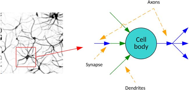
layer consists of a single instance or entry of our training data—such as a single image of a dog or a cat,
where each neuron is a number representing the color of each pixel in the image—while the output layer
can be thought of as the desired output of our network—such as the classification “dog” or “cat.” Again,
the idea is we’re making a mapping from our data to a result, and the network is using many examples of
training data to make the best possible mapping.

                                                                                 That’s a cat!

2.2 Neurons
How does the network actually go about making this mapping from data to a desired output? It’s time
we take a closer look at the fundamental units of artificial neural networks: Neurons.

In the brain, biological neurons are highly connected and communicate chemical signals through
synapses between axons and dendrites. The human brain is estimated to have 100 billion neurons,
with each neuron connected to up to 10,000 other neurons.

© 2021 IBM Corporation                                                                                   7
So how do artificial neurons compare? For the moment, you can think of artificial neurons simply as
stores of values between 0 and 1—analogous to those chemical signals in biological neurons. A neuron
with a corresponding value of 1 is said to be “activated,” like a firing neuron in the brain passing its
signal on to another neuron, while a neuron with a corresponding value of 0 is said to inactive.
Consider how an input image (like the one of the cat up there) can then be represented as a collection of
neurons. We assign each pixel in the image a number between 0 and 1 depending on its coloration, or
activation.
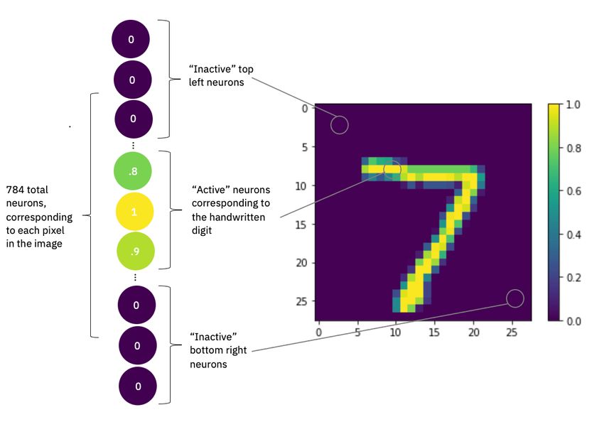
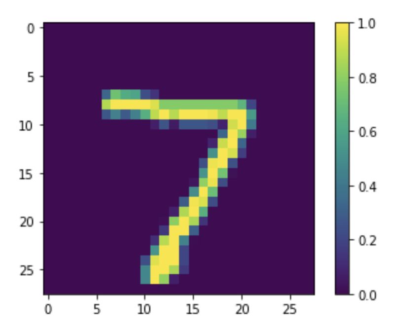
To see this more clearly, let’s look at one of the handwritten digit images we’ll be looking at in our
coding exercise for this lab.
The image consists of 28x28 pixels, meaning there
are 784 pixels in total. Notice how the pixels on the
actual “7” are lit up yellow, corresponding with
number close to or equal to 1, while pixels that don’t
have any “7” on them are equal to 0, meaning they’re
not activated at all.
Now, imagine a column of 784-pixel neurons—again,
for now just values between 0 and 1—starting from
the top left pixel in the image to bottom right. This is
how we’d represent this data entry, the digit “7,” in
the input layer of a neural network.
© 2021 IBM Corporation 8
2.3 Layers
Now that we’ve seen how we represent the information in our data in terms of active and inactive
neurons. The stacking of these neurons—which we visually depict as a column—represents a “layer.”
These layers create an ordered sequence for our network, where information “feeds forward” from the
input layer to the output layer. In truth, there are a wide variety of different neural network
architectures which vary the number, size, and order of layers, but for our purposes we’ll be focusing on
the basic feed forward architecture.

When looking at our neural network diagram, you may be wondering why the output layer is smaller (i.e.
it consists of fewer neurons) than our input layer (our original pixel neurons). Recall that ultimately, our
network is trying to build a mapping from the input (data) to the output, which is whatever we’re
interested in making the neural network do. So, in a task like classifying handwritten digits, that means
that the output layer neurons actually correspond to the neural network’s prediction for what a
particular digit is.

                                                                           Let’s imagine we’re trying to
                                                                           get our network to map our
                                                                           digits to one of three
                                                                           numbers: 7, 8, or 9. In other
                                                        Three possible
                                                                           words, we want the network
                                                         classifications
                                                                           to tell us whether the
                                                            /outputs
                                                                           handwriting we’re showing it
                                                                        7 is a 7, 8, or a 9. Those 3
                                                                           neurons in the output layer
                                                                           each correspond to one of
                                                                        8 those numbers. And after the
                                                                           network has received signals
                                                                           (numbers) from the
                                                                        9
                                                                           preceding hidden layers—all
                                                                           the way back to our original
                                                                           input digit layer, it too will
                                                                           assign a value between 0 and
                                                                           1 to each of those final 3
neurons. Whichever neuron has the highest value (activation), will correspond with the networks
decision on what the digit is!

© 2021 IBM Corporation                                                                                     9
Winner! That
.9 7
digit is a 7!
.1 8
.2 9
What of the intermediate, “hidden” layers? Again, the network is feeding forward signals from the
original input layer to the output classification. Therefore, those signals are actually being passed and
transformed through the intermediate “hidden” layers composed also of neurons taking on values
between 0 and 1. We can think of these hidden layers as possible “pathways” for our network to use as
it tries to make the best possible mapping from input to output. The number of hidden layers as well as
the numbers of neurons they contain is actually something that we the data scientist can control and
change. In practice, finding the best architecture for the network to perform its task can be a process of
experimentation, trial, and error.
Recall that our input layer corresponds with the pixels in our starting image. What do the hidden layers
correspond with? It turns out it’s not always easy to intuit what the hidden layers actually represent in
the “mind” of our artificial neural network. If we were to visualize them—again drawing an image based
on the activations of the individual pixels—the hidden layers may look something like these:
We call these “latent” representations of our data. They’re the way that our network “learns” the latent
features associated with the digits. The network sees an input, maps it through the hidden layer latent
spaces, and ultimately produces values for our output layer corresponding with what it believes the digit
to be. When you think about it, this is much like how our own brains may process these same data. Even
if we don’t realize it, our brains tell digits apart by sending signals corresponding with the features they
contain. A circular shape in the digit (potentially captured by one hidden layer) might point your brain to
a “0” or an “8.” Two circular shapes in the image (potentially captured by two hidden layers) would be a
© 2021 IBM Corporation 10strong indicator of an “8.” Of course, this all happens subconsciously for us—in a sense the process is
“hidden” to us. Hence, the intermediate “hidden” layers of the artificial neural network. The particular
combinations of activations in the latent hidden layers are ultimately what allows the network to make
its mapping from input to output.
2.4 Connecting Neurons
The final component of our
neural network that we
haven’t yet discussed are the
connections between the
layers of neurons. Notice how
each neuron has lines
connected to all of the
neurons in the previous layer,
as well connections to all of
the neurons in the following
layer. Intuitively, this is how
activating signals feed
forward through the network.
In a fully connected or
“dense” neural network,
such as the ones we’ll be
dealing with in this lab, each
neuron receives information
from every neuron in the
preceding layer. Likewise, it passes on information to every neuron in the succeeding layer. Remember
that every neuron throughout the network takes on a value between 0 and 1. Apart from the input layer
(which takes its values from the original input image), each other neuron will be assigned a value
according to the information it’s receiving from the previous layer’s neurons.
The mechanism by which a neuron’s activation is determined—based on the sum of all the information
from the previous layer—is a mathematical function of what are known as “weights” and “biases” which
compose the connections between neurons. This is the only formula we’ll be dealing with in this lab, and
it’s okay if you don’t recognize some of the symbols that it contains.
For now, just know that the left side of the equation represents the actual activation of each neuron—the
value we assign to it—so, as we’ve seen, a number between 0 and 1. That value is equal to the right side
of the equation, which we can think of as existing in each and every one of the connections between
neurons in our network. On this right-hand side, the X terms, i.e. X1, X2, and X3 represent the values of
the neurons feeding into our new neuron. Meanwhile the W terms, i.e. W1, W2, and W3, correspond with
the “weights” or “importances” the network assigns each of those preceding activation values. For the
© 2021 IBM Corporation 11moment, you can ignore the “bias” term on both sides of the equation—this term just seeks to constrain
the ultimate output of the equation to ensure it leads to a value between 0 and 1.
In this case, we’re calculating a neuron based on information from 3 neurons in the previous layer,
hence 3 X terms and 3 W terms. If we were to zoom in on such a neuron it might look something like
this:
W1
W2
W3
Therefore, a neuron’s activation is calculated as the sum of all of the previous neuron activations,
multiplied by the weights that the network has assigned to them, plus some bias term.2 And this value in
turn becomes a new X1 (or X2 or X3) that gets input into the following layer, all the way until the output
layer when a final result is produced.
So, what really are these weights assigned to the values of neurons as they send their signal to the next
layer? You can think of them again as “importances”—or how important our network believes each
signal should be in determining the value of a receiving neuron. If a weight has a low value, that means
the network believes it is relatively unimportant in determining the next neuron (thus, a smaller W term
means that the whole product will be smaller as well). And vice versa, a higher weight indicates that the
network assigns a lot of importance to this particular signal.
2.5 Learning the Right Weights
Recall that we have been thinking about neurons and layers as the potential pathways a neural network
can use to make a mapping from a particular input to a (hopefully) correct output. Ultimately, then, we
2
In practice, there is an additional step whereby the output is “squished” through a given “activation
function” to ensure the value ends up between 0 and 1, but we don’t need to worry about that for now.
© 2021 IBM Corporation 12can think of the weights of the neural network as the actual pathway that the network ends up choosing.
In other words, weights are the way the network actually builds a route to send information through the
layers and neurons to an output.
But how does the network know which weights to use? Remember that each connection from one
neuron to another carries with it an assigned weight. That means that for just two layers each consisting
of 784 neurons, the network will have to assign 784 * 784 = 614,656 weights! The process of finding the
optimal values for these weights, such that the network is as effective as possible in making correct
predictions, is where the “learning” part of Deep Learning comes in. The precise mathematical process
whereby this happens is beyond the scope of this lab. However, the intuition behind what’s going on is
surprisingly simple.
Essentially, the “training” of a neural network with “training data”—the data the network uses to learn—
is the process of allowing the network to try many different combinations of weights between its
neurons and layers and adjusting them in a way that makes its ultimate predictions as accurate as
possible on the “test data”—the data we use to test how good the network is at the task. More
specifically, the network is trying to tweak the weights in such a way that it minimizes its “loss”–a
numerical representation of how wrong it is in making its predictions. For example, if the network
predicts 60% of the images in the test data correctly, then it’s loss might be something like 0.4.3 If it
predicts 65% correctly, the loss might then be 0.35. The network’s goal is to choose weights such that
the loss is as low as possible, i.e. it is as accurate as possible in making its predictions.
We can visualize this process with a diagram
like this one. The Y-axis is the overall loss,
which is again the measure of “how wrong”
the neural network was in its predictions.
The X-axis is the value of a particular weight
for the connection between two neurons
somewhere in the network.
Notice how at the “Starting point”—the
network’s first try at predicting the test
images—the loss is quite high. This means
the network didn’t do a very good job of
predicting the digits.4 Each subsequent
point on the line represents the network’s
next attempt at predicting the test data,
after it has gone about incrementally
changing the value of the weight. Each of
these iterations, whereby the network
updates its mapping with new weights, is
known as a “training epoch”—which is
3
We say “something like” here because there are a number of different approaches to calculating the
loss in a neural network, which we call “loss functions,” and these will affect what the precise loss value
is.
4
In most cases, the initial weights used across the neural network, i.e. before any training has begun,
are assigned randomly, which is why the loss is quite high. In practice, other strategies are sometimes
used to set the starting weights in a process known as “weight initialization.”
© 2021 IBM Corporation 13simply a pass through the training data. In this simple example, the network is only running through seven training epochs (corresponding with the seven points on the blue curve). In practice, neural networks may go through hundreds, thousands, or even millions of training epochs depending on their complexity. Regardless of how many epochs are used, the network’s goal is to “descend” down the “gradient” of this loss function until it finally converges to a point where the loss or “cost function” is minimized (as small as possible). This is the process of “gradient descent”—the main mechanism by which neural networks learn using data! Neural networks learn by conducting immense gradient descent optimizations across thousands, millions, and sometimes even billions of weights. Furthermore, although we’re using a simple two- dimensional diagram to depict this process, in reality neural networks conduct this optimization process with respect to more than one weight in each training epoch. In other words, the network is trying to find the minimum possible loss for some function involving N number of weights. That N controls the dimensionality of the loss function—which we can’t really visualize once it goes beyond three! Recall our earlier discussion about the fact that neural networks are computationally expensive—hopefully this section has put that truth into greater perspective. © 2021 IBM Corporation 14
3 Glossary and Conclusion
Artificial Intelligence: The design and building of intelligent agents (computer systems) that take
information from an environment (data) and use it to take actions that affect that environment

Machine Learning: The study of computer algorithms that improve automatically through experience
and by the use of data

Deep Learning: The subfield of Machine Learning focusing on building artificial neural networks to train
systems to accomplish complex tasks; The technology underlying many of the most successful AI
applications, such as self-driving cars

Artificial Neural Networks (Neural Networks): The fundamental approach in Deep Learning; Computer
algorithms aimed at mimicking the ways that biological brains send information across brain cells
(neurons) as part of information processing. They consist primarily of layers of artificial “neurons” and
the connections between them

Feed-Forward Neural Networks: Neural networks which pass information forward from a starting
“input layer” to an ultimate “output layer” (without cycling backwards at any point in the process); The
oldest and most fundamental neural network “architecture”

Artificial Neurons (Neurons): A store or “node” of information in a neural network, generally calculated
according to signals received from connected neurons in a previous layer

Layers: A series of neurons representing one step during the sequential processing of a neural network;
an architectural parameter of neural networks

Input Layer: The left-most “starting layer” in a neural network, corresponding with instances of training
data

Output Layer: The right-most “final layer” in a neural network, corresponding with the network’s final
prediction or classification, e.g. which digit is contained in an image provided in the input layer

Classification: In Machine and Deep Learning, the algorithmic task of predicting class labels for given
examples of input data, where classes may be categories such as “dog or cat” or “digits between 0 and
9.”

Hidden Layer(s): Intermediate layers in a neural network between the input and output layers,
representing latent features used by the network to perform its given task

Training Data: Data used to train neural networks and other machine learning algorithms; Used by
neural networks to conduct gradient descent when attempting to minimize overall loss for a particular
task

Testing Data: Data used to test the performance of a trained neural network

Loss: Quantitative measure of overall “wrongness” in the outputs of a neural network; Calculated using
a variety of “loss functions” chosen by the data scientist depending on the task

© 2021 IBM Corporation                                                                                   15
Training Epoch: A neural network’s single pass through of a training dataset, after which weights are
adjusted to minimize overall loss; A parameter that we as the developer choose—most neural networks
train over the course of many epochs, but we may vary this process depending on the data and the task
at hand

Weights: “Importances” assigned to the signals being sent from one neuron to another in a neural
network; Values that make up the actual “mapping” of a neural network from input to output, through
hidden layers, and optimized through gradient descent across training epochs

Gradient Descent: A mathematical algorithm whereby neural networks attempt to find given weights to
assign throughout the network that minimize the overall loss for a task; The attempted “descent” down
the curve of a function to a convergent minimum

Weight Initialization: The strategy whereby weights are assigned in a neural network prior to any
training; Usually done randomly, but sometimes other strategies are used

IBM Watson Studio: IBM’s cloud-based Integrated Development Environment (IDE) for Data Science
and AI

Python: A high-level, general-purpose programming language preferred by many Data Scientists and AI
Engineers because of its associated libraries

TensorFlow: A free and open-source Python library developed by Google primarily focused on Deep
Learning; Preferred by many Data Scientists and AI Engineers for building neural networks

Keras: A free and open-source Python library developed by Google engineer François Chollet that
provides an easier-to-use interface for programming with TensorFlow

3.1 Where to Go Next
If you’re interested in looking closer at Deep Learning and neural networks, such as into the
mathematics weight calculation, optimization through various forms of gradient descent, and how all of
this can change in different types of neural networks (different “architectures”), we encourage you to
take a look at course five of IBM’s Machine Learning Professional Certificate on Coursera.

Here are a few more consolidated resources on the topics we’ve discussed in this lab that you can find
on IBM’s developer community:

    •   Watson Studio

    •   AI Beginner’s Guide

    •   Neural Networks

    •   Deep Learning

    •   Gradient Descent

© 2021 IBM Corporation                                                                                16
You can also read