Predicting the Present with Google Trends
←
→
Page content transcription
If your browser does not render page correctly, please read the page content below
Predicting the Present with Google Trends
                            Hyunyoung Choi, Hal Varian∗
                                    December 18, 2011

                                            Abstract
        In this paper we show how to use search engine data to forecast near-term values
        of economic indicators. Examples include automobile sales, unemployment claims,
        travel destination planning, and consumer confidence.

Government agencies periodically release indicators of the level of economic activity in
various sectors. However, these releases are typically only available with a reporting lag
of several weeks and are often revised a few months later. It would clearly be helpful to
have more timely forecasts of these economic indicators.
    Nowadays there are several sources of data on real-time economic activity available
from private sector companies such as Google, MasterCard, Federal Express, UPS, Intuit
and many others. In this paper we examine Google Trends, which is a a real-time daily
and weekly index of the volume of queries that users enter into Google. We have found
that these query indices are often correlated with various economic indicators and may
be helpful for short-term economic prediction.
    We are not claiming that Google Trends data can help in predicting the future. Rather
we are claiming that Google Trends may help in predicting the present. For example, the
volume of queries on automobile sales during the second week in June may be helpful in
predicting the June auto sales report which is released several weeks later in July.
    It may also be true that June queries help to predict July sales, but we leave that
question for future research, as this depends very much on the particular time series in
question. We have found that queries can be useful leading indicators for subsequent
consumer purchases in situations where consumers start planning purchases significantly
in advance of their actual purchase decision.
    Predicting the present, in the sense described above, is a form of “contemporaneous
forecasting” or “nowcasting,” a topic which is of particular interest to central banks and
other government agencies. As Castle et al. [2009] point out, contemporaneous forecast-
ing is valuable in itself, but it also raises a number of interesting econometric research
questions involving topics such as variable selection, mixed frequency estimation, and
incorporation of data revisions, to name just a few.
    Our goals in this paper are to familiarize readers with Google Trends data, illustrate
some simple forecasting methods that use this data, and encourage readers to undertake
their own analyses.
  ∗
      hal@google.com

                                               1
We do not claim any methodological advances here; certainly it is possible to build
more sophisticated forecasting models than those we use. However, we believe that the
models we describe can serve as baselines to help analysts get started with their own
modeling efforts and that can subsequently be refined for specific applications.1
Our examples use R, a freely available open-source statistics package from http://
CRAN.R-project.org. We provide the R source code and data in the online appendix
available at http:tobeprovided.
1 Literature review
So far as we know, the first published paper that suggested that web search data was
useful in forecasting economic statistics was Ettredge et al. [2005], which examined the
U.S. unemployment rate. At about the same time Cooper et al. [2005] described using
internet search volume for cancer-related topics. Since then there have been several papers
that have examined web search data in various fields.
For example, in the field of epidemiology, Polgreen et al. [2008] and Ginsberg et al.
[2009] showed that search data could help predict the incidence of influenza-like diseases.
This work was widely publicized and stimulated several further findings in epidemiology,
including Brownstein et al. [2009], Corley et al. [2009], Hulth et al. [2009], Pelat et al.
[2009], Valdivia and Monge-Corella [2010], and Wilson [2009].
In economics, Choi and Varian [2009a,b] described how to use Google Search Insights
data to predict several economic metrics including initial claims for unemployment, au-
tomobile demand, and vacation destinations; this report is an updated and streamlined
version of those working papers. Askitas and Zimmermann [2010], D0 Amuri and Mar-
cucci [2010], and Suhoy [2009] examined unemployment in the US, Germany and Israel.
Guzman [2011] has examined Google data as a predictor of inflation.
Recently, Baker and Fradkin [2011] have used Google search data to examine how job
search responded to extensions of unemployment payments.
Radinsky et al. [2009], Huang and Penna [2009], and Preis et al. [2010] examine the
use of search data for measuring consumer sentiment while Schmidt and Vosen [2009] and
Lindberg [2011] examine retail sales and consumption metrics. Wu and Brynjolfsson [2010]
examine housing data using longitudinal data extracted from Google Search Insights.
Shimshoni et al. [2009] describe the predictability of Google Trends data itself, pointing
out that a substantial amount of search terms are highly predictable using simple seasonal
decomposition methods.
Goel et al. [2010] provide a useful survey of work in this area and describe some of
the limitations of web search data. As they point out, search data is easy to acquire
and is often helpful in making forecasts, but may not provide dramatic increases in pre-
dictability. Although we generally agree with this view, we typically find economically
significant, if not dramatic, improvements in forecast performance using search engine
data, as illustrated in this paper.
1
This paper is a much simplified and streamlined version of our earlier working papers, Choi and
Varian [2009a,b] which includes other more sophisticated models.
2Finally, McLaren and Shanbhoge [2011] summarize how web search data can be used
for economic nowcasting by central banks.
2 Google Trends
Google Trends provides a time series index of the volume of queries users enter into Google
in a given geographic area.
The query index is based on query share: the total query volume for the search term
in question within a particular geographic region divided by the total number of queries
in that region during the time period being examined. The maximum query share in the
time period specified is normalized to be 100 and the query share at the initial date being
examined is normalized to be zero.
The queries are “broad matched” in the sense that queries such as [used automobiles]
are counted in the calculation of the query index for [automobile]. The data go back to
January 1, 2004.
Note that Google Trends data is computed using a sampling method and the results
therefore vary a few percent from day to day. Furthermore, due to privacy considerations,
only queries with a meaningful volume are tracked. There is a substantial amount of
online help available via links on the site which describe details of how of how the data is
collected.
This query index data is available at country, state, and metro level for the United
States and several other countries. There are two user interfaces for the data, Google
Trends and Google Insights for Search (I4S). The latter is the more useful for our purposes
since it allows a logged-in user to download the query index data as a CSV file.
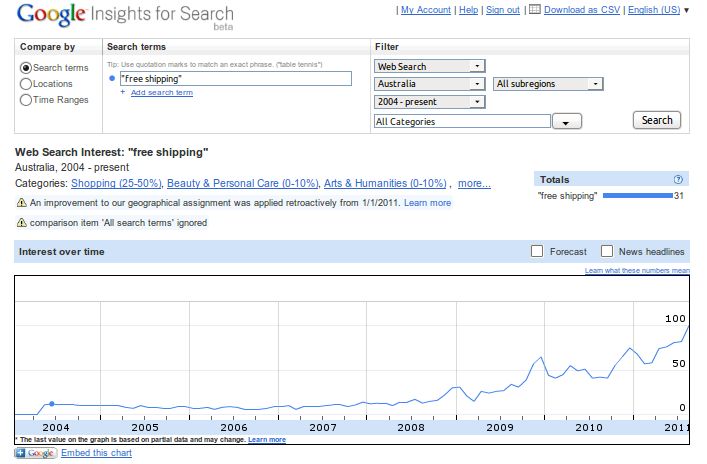
Figure 1 depicts example output from I4S for the query [free shipping] in Australia.
The search share for this query has exhibited significant increase since 2008 and tends to
peak during the holiday shopping season.
Google classifies search queries into about 30 categories at the top level and about 250
categories at the second level using a natural language classification engine. For example,
the query [car tire] would be assigned to category Vehicle Tires which is a subcategory
of Auto Parts which is a subcategory of Automotive. The assignment is probabilistic
in the sense that a query such as [apple] could be partially assigned to Computers &
Electronics, Food & Drink, and Entertainment.
3 Examples
3.1 Motor vehicles and parts
As an initial example we use the “Motor Vehicles and Parts Dealers” series from the U.S.
Census Bureau “Advance Monthly Sales for Retail and Food Services” report.2
This index summarizes results from a survey sent to motor vehicle and parts dealers
that asks about current sales. The preliminary index is released 2 weeks after the end of
2
http://www.census.gov/retail/marts/www/timeseries.html.
1Figure 1: Search index for [free shipping] in Australia
each month. The data is available in both seasonally adjusted and unadjusted form; here
we use the unadjusted data.
Let yt be the log of the observation at time t. We first estimate a simple baseline
seasonal AR-1 model yt = b1 yt−1 + b12 yt−12 + et for the period 2004-01-01 to 2011-07-01.
Estimate Std. Error t value Pr(>|t|)
(Intercept) 0.67266 0.76355 0.881 0.381117
lag(y, -1) 0.64345 0.07332 8.776 3.59e-13 ***
lag(y, -12) 0.29565 0.07282 4.060 0.000118 ***
---
Multiple R-squared: 0.7185,Adjusted R-squared: 0.7111
Google Trends contains several automotive-related categories. We use the searches
from the first Sunday-Saturday contained in the month, which gives us a 4-6 week fore-
casting lead. A little experimentation shows that two of these categories, Trucks & SUVs
and Automotive Insurance significantly improve in-sample fit when added to this re-
gression.
Estimate Std. Error t value Pr(>|t|)
(Intercept) -0.45798 0.78438 -0.584 0.561081
lag(y, -1) 0.61947 0.06318 9.805 5.09e-15 ***
lag(y, -12) 0.42865 0.06535 6.559 6.45e-09 ***
suvs 1.05721 0.16686 6.336 1.66e-08 ***
insurance -0.52966 0.15206 -3.483 0.000835 ***
---
Multiple R-squared: 0.8179,Adjusted R-squared: 0.808
2However, the perils of in-sample forecasting are well-known. The question of interest
is whether the Trends variables improve out-of-sample forecasting.
To check this, we use a rolling window forecast where we estimate the model using
the data for periods k through t − 1 and then forecast yt using yt−1 , yt−12 , and the
contemporaneous values of the Trends variables as predictors. Since the series is actually
released 2 weeks after the end of each month, this gives us a meaningful forecasting lead.
The value of k is chosen so that there are a reasonable number of observations for the
first regression in the sequence. In this case we chose k = 17, which implied the forecasts
start in 2005-06-01.
The results are shown in Figure 2. The mean absolute error of log(yt ) using the
baseline seasonal AR-1 model is 6.34% while the MAE using the Trends data is 5.66%,
an improvement of 10.6%. If we look at the MAE during the recession (December 2007
through June 2009) we find that the MAE without Trends data is 8.86% and with Trends
data is 6.96%, an improvement of 21.4%.
Motor Vehicles and Parts
11.4
actual
base
trends
11.2
log(mvp)
11.0
MAE improvement
10.8
Overall = 10.5%
During recession = 21.5%
2006 2007 2008 2009 2010 2011
Index
Figure 2: Motor Vehicles and Parts
3.2 Initial claims for unemployment benefits
Each Thursday morning the US Department of Labor releases a report describing the
number of people who filed for unemployment benefits in the previous week.3
Initial claims have a good record as a leading indicator. Macroeconomist Robert
Gordon indicates that there is a “surprisingly tight historical relationship in past US re-
cessions between the cyclical peak in new claims for unemployment insurance (measured
3
http://www.dol.gov/opa/media/press/eta/ui/current.htm
3as a four-week moving average) and the subsequent NBER trough.”4 Furthermore, a cur-
sory inspection of relationship between initial claims and the unemployment rate indicates
that initial claims tend to peak 12–18 months before the unemployment rate peaks.
When someone becomes unemployed it is natural to expect that they will issue searches
such as [file for unemployment], [unemployment office], [unemployment benefits], [un-
employment claim], [jobs], [resume] and so on. Google Trends classifies search queries
like these into two categories, Local/Jobs and Society/Social Services/Welfare &
Unemployment.
In this example we work with the seasonally adjusted initial claims data, since that is
the number used by most economic forecasters. Since our dependent variable is seasonally
adjusted, it makes sense to seasonally adjust the independent variables as well, so we used
the stl command in R to remove the seasonal component of the Trends data.
In this case, our baseline regression is a simple AR-1 model on the log of initial claims.
Start = 2004-01-17, End = 2011-07-02
Estimate Std. Error t value Pr(>|t|)
(Intercept) 0.25488 0.12951 1.968 0.0498 *
L(y, 1) 0.98022 0.01007 97.368 |t|)
(Intercept) 1.0563440 0.2686360 3.932 9.98e-05 ***
L(y, 1) 0.9183560 0.0208778 43.987 < 2e-16 ***
Jobs 0.0007069 0.0003847 1.838 0.0669 .
Welfare...Unemployment 0.0003752 0.0001838 2.042 0.0418 *
---
Multiple R-squared: 0.962,Adjusted R-squared: 0.9618
When we look at one-step-ahead out-of-sample forecasts we find that the MAE goes
from 3.37% using the baseline forecast to 3.68% using the Trends data which is a 5.95%
reduction in fit. However, when we look at the series a bit more closely a rather different
picture emerges.
It is well-known that it is difficult to identify “turning points” in economic series. A
smoothly increasing or decreasing trend is easy to fit with a simple linear AR model.
Turning points in time series are much harder to forecast.
4
See http://www.voxeu.org/index.php?q=node/3524 for details
4start end MAE base MAE trends 1-ratio
2009-03-01 2009-05-01 0.0306 0.02398 21.85%
2009-12-01 2010-02-01 0.0356 0.03127 12.36%
2010-07-15 2010-07-15 0.0513 0.05101 0.65%
2011-01-01 2011-05-01 0.0252 0.02446 3.22%
Table 1: Behavior of MAE around turning points.
If we look just at the recession period (December 2007 through June 2009) we find
that using Trends data reduces the MAE from 3.98% to 3.44%, an improvement of 13.6%.
Looking more closely at the series, we see that there are four notable turning points
indicated by the shaded areas in Figure 3. The MAE for the period surrounding these
turning points are reported in Table 1. Note that there is a reduction in MAE at all
turning points, with particularly pronounced reductions in the first two. In this case, the
Google Trends data seems to help in identifying at least two of the turning points in the
series.
Initial claims SA
13.4
13.2
log(iclaims)
13.0
12.8
2009 2010 2011
time
Figure 3: Seasonally adjusted initial claims for unemployment; turning points in gray.
Figure 4 plots the difference in MAE for the Base and Trends model. A positive value
indicates that the Trends forecast had a smaller error. Here it is clear that Trends model
fits better during the recession (December 2007 through June 2009), while the Base fits
better immediately after.
5Base − trends absolute forecast error
0.04
diff error
0.00
−0.04
−0.08
2008 2009 2010 2011
Time
Figure 4: Base absolute error – Trends absolute error.
Askitas and Zimmermann [2010], Suhoy [2009], and D0 Amuri and Marcucci [2010] have
confirmed the value of search data in forecasting unemployment in the U.S., Germany and
Israel.
3.3 Travel
The internet is commonly used for travel planning which suggests that Google Trends data
about destinations may be useful in predicting visits to that destination. We illustrate
this using data from the Hong Kong Tourism Board.5
The Hong Kong Tourism Board publishes monthly visitor arrival statistics, including
“Monthly visitor arrival summary” by country/territory of residence. For this study we
use visitor data from US, Canada, Great Britain, Germany, France, Italy, Australia, Japan
and India.
“Hong Kong” is also one of the subcategories in under Vacation Destinations in Google
Trends. We can examine the query index for this category by country of origin.
The Hong Kong visitor arrival data is not seasonally adjusted, nor is the Google Trends
data. We used the average query index in the first two weekly observations of the month
to predict the total monthly visitors. Since the data is released with a one-month lag,
this gives us roughly a 6-week lead in terms of forecasting
We let yt be the visitors from a given country in month t, and xt be the average
Google Trends index for Vacation Destinations/Hong Kong for the first two weeks of
that month. We can specify a basic seasonal AR-1 model of the form yt = b1 yt−1 +
b12 yt−12 + b0 xt + et .
We estimate this model for each country and compare the actual to the fitted results
in Figure 5. Unlike the previous examples, we have here used in-sample fits. As can be
5
http://partnernet.hktourismboard.com
6seen, the in-sample fits are pretty good, with the exception of Japan. Excluding Japan,
the average R2 is 73.3%. In Choi and Varian [2009a] we use a more elaborate random
effects model with some additional predictors and find a somewhat better in-sample fit.
US CA GB
60000
110000
35000
visitors
visitors
70000
20000
30000
2005 2007 2009 2011 2005 2007 2009 2011 2005 2007 2009 2011
DE
date
FR
date
IT
date
25000
12000
20000
visitors
visitors
15000
6000
10000
2005 2007 2009 2011 2005 2007 2009 2011 2005 2007 2009 2011
AU
date
JP
date
IN
date
60000
20000 50000
110000
visitors
visitors
30000
70000
2005 2007 2009 2011 2005 2007 2009 2011 2005 2007 2009 2011
Figure 5: Visitors to Hong Kong
4 Consumer confidence
In our final example, we examine the Roy Morgan Consumer Confidence Index for Aus-
tralia.6 Unlike our earlier examples, it is not obvious what categories would be most
helpful in predicting this series. There are a variety of methods one can use for variable
selection; see Castle et al. [2010] for a recent discussion of this topic with emphasis on
nowcasting applications.
We used a Bayesian method known as “spike and slab” regression first described by
George and McCulloch [1997]. This technique produces a posterior probability that a
variable enters a regression (i.e., has a non-zero coefficient) along with an estimate of that
coefficient’s posterior distribution.
We used Google Trends category data for Australia, taking the average value of the
category data for the first two weeks of the month and seasonally adjusting it using the R
command stl. The spike and slab technique assigned high posterior probabilities to the
categories Crime & Justice, Trucks & SUVs, and Hybrid & Alternative Vehicles.
The last two are not surprising as they are highly correlated with the price of gasoline,
6
http://www.roymorgan.com/news/polls/consumer-confidence.cfm
7which is known to impact consumer confidence in the United States. We have no expla-
nation for the first predictor. Plotting the Crime & Justice time series shows a definite
correlation with consumer confidence for the period we examine, but of course there is no
way to know if this correlation will persist in the future.
Our predictor for Australian log(consumer confidence) is summarized in this table.
Estimate Std. Error t value Pr(>|t|)
(Intercept) 1.5172617 0.2795356 5.428 5.67e-07 ***
lag(y, -1) 0.6839436 0.0584158 11.708 < 2e-16 ***
Crime...Justice -0.0009664 0.0002404 -4.020 0.000129 ***
Trucks...SUVs 0.0010600 0.0005346 1.983 0.050735 .
Hybrid...Alternative.Vehicles -0.0007869 0.0001482 -5.308 9.26e-07 ***
---
Multiple R-squared: 0.8583,Adjusted R-squared: 0.8514
The Trends predictors reduce MAE of the simple AR-1 model by about 12.7% for
in-sample forecasts. One-step-ahead MAE goes from 3.63% to 3.29%, an improvement of
9.3%; see Figure 6. The big drop in Spring 2008 is due to a significant increase in queries
on Hybrid & Alternative Vehicles which is likely due to the increased price of oil that
occurred during that period.
Roy Morgan Consumer Confidence for Australia
4.9
4.8
4.7
log(conf)
4.6
4.5
actual
MAE improvement base
Overall = 9.5% trends
4.4
2005 2006 2007 2008 2009 2010 2011
Index
Figure 6: Australia consumer confidence.
5 Conclusion
We have found that simple seasonal AR models that include relevant Google Trends
variables tend to outperform models that exclude these predictors by 5% to 20%. We
8hope that these examples will encourage other researchers to experiment this data source
in their own research.
Google Trends data is available at a state and metro level for several countries. We
have also had success with forecasting various business metrics using state-level data. It
some cases longitudinal data helps make up for the rather short time series available from
Google Trends.
9References
Nikos Askitas and Klaus F. Zimmermann. Google econometrics and unemployment fore-
casting. Technical report, SSRN 899, 2010. URL http://papers.ssrn.com/sol3/
papers.cfm?abstract_id=1465341.
Scott Baker and Andry Fradkin. What drives job search? Evidence from Google search
data. Technical report, Stanford University, 2011. URL http://papers.ssrn.com/
sol3/papers.cfm?abstract_id=1811247.
John S. Brownstein, Clark C. Freifeld, and Lawrence C. Madoff. Digital disease
detection—harnessing the web for public health surveillance. New England Journal of
Medicine, 2009. URL http://www.ncbi.nlm.nih.gov/pmc/articles/PMC2917042/.
Jennifer L. Castle, Nicholas W. P. Fawcett, and David F. Hendry. Nowcasting is not
just contemporaneous forecasting. National Institute Economic Review, 201(1):71–89,
October 2009. URL http://ner.sagepub.com/content/210/1/71.abstract.
Jennifer L. Castle, Nicholas W. P. Fawcett, and David F. Hendry. Evaluating automatic
model selection. Technical Report 474, Department of Economics, University of Oxford,
2010. URL http://economics.ouls.ox.ac.uk/14734/1/paper474.pdf.
Hyunyoung Choi and Hal Varian. Predicting the present with Google Trends. Tech-
nical report, Google, 2009a. URL http://google.com/googleblogs/pdfs/google_
predicting_the_present.pdf.
Hyunyoung Choi and Hal Varian. Predicting initial claims for unemployment insurance us-
ing Google Trends. Technical report, Google, 2009b. URL http://research.google.
com/archive/papers/initialclaimsUS.pdf.
C. Cooper, K. Mallon, S. Leadbetter, L. Pollack, and L. Peipins. Cancer internet search
activity on a major search engine, United States 2001-2003. J Med Internet Res, 7,
2005. URL http://www.ncbi.nlm.nih.gov/pmc/articles/PMC1550657/.
C. D. Corley, A. R. Mikler, K. P. Singh, and D. J. Cook. Monitoring influenza trends
through mining social media. Proceedings of the 2009 International Conference on
Bioinformatics and Computational Biology (BIOCOMP09), 2009. URL http://eecs.
wsu.edu/~cook/pubs/biocomp09.pdf.
Francesco D0 Amuri and Juri Marcucci. Google it! Forecasting the US unemployment rate
with a Google job search index. SSRN, 2010. URL http://papers.ssrn.com/sol3/
papers.cfm?abstract_id=1594132.
M. Ettredge, J. Gerdes, and G. Karuga. Using web-based search data to predict
macroeconomic statistics. Communications of the ACM, 48(11):87–92, 2005. URL
http://portal.acm.org/citation.cfm?id=1096010.
E. I. George and R. E. McCulloch. Approaches for Bayesian variable selection. Statistica
Sinica, 7:339–374, 1997.
10Jeremy Ginsberg, Matthew H. Mohebbi, Rajan S. Patel, Lynnette Brammer, Mark S.
Smolinski, and Larry Brilliant. Detecting influenza epidemics using search engine query
data. Nature, pages 1012–1014, 2009. URL http://research.google.com/archive/
papers/detecting-influenza-epidemics.pdf.
Sharad Goel, Jake M. Hofman, Sébastien Lahaie, David M. Pennock, and Duncan J.
Watts. Predicting consumer behavior with web search. Proceedings of the National
Academy of Sciences, 7(41):17486–17490, Sep 27 2010. doi: 10.1073/pnas.1005962107.
URL http://www.pnas.org/content/early/2010/09/20/1005962107.
Giselle Guzman. Internet search behavior as an economic forecasting tool: the case of
inflation expectations. The Journal of Economic and Social Measurement, September
2011. Forthcoming.
Haifang Huang and Nicolas Dell Penna. Constructing consumer sentiment index for U.S.
using Google searches. Technical report, University of Alberta, 2009. URL http:
//econpapers.repec.org/paper/risalbaec/2009_5f026.htm.
A. Hulth, G. Rydevik, and A. Linde. Web queries as a source for syndromic surveillance.
PLoS ONE, 4, 2009. URL http://www.plosone.org/article/info:doi/10.1371/
journal.pone.0004378.
Fredrik Lindberg. Nowcasting Swedish retail sales with Google search query data. Master’s
thesis, Stockholm University, 2011. URL http://www.ne.su.se/education/master/
econ_master/year2_thesis/theses/02_lindberg_f.pdf.
Nick McLaren and Rachana Shanbhoge. Using internet search data as economic indicators.
Bank of England Quarterly Bulletin, June 2011. URL http://www.bankofengland.
co.uk/publications/quarterlybulletin/qb110206.pdf.
Charles R. Nelson and Charles I. Plosser. Trends and random walks in macroeconomic
time series: Some evidence and implications. Journal of Monetary Economics, 10:
132–162, 1982.
C. Pelat, C. Turbelin, A. Bar-Hen, A. Flahault, and A-J. Valleron. More diseases tracked
by using Google Trends. Emerg Infect Dis., 15:1327–8, 2009. URL http://www.cdc.
gov/eid/content/15/8/1327.htm.
P. M. Polgreen, Y. Chen, D. M. Pennock, and F. D. Nelson. Using internet searches for
influenza surveillance. Clinical Infectious Diseases, 47:1443–1448, 2008. URL http:
//www.ncbi.nlm.nih.gov/pubmed/18954267.
Tobias Preis, Daniel Reith, and H. Eugene Stanley. Complex dynamics of our economic
life on different scales: insights from search engine query data. Phil. Trans. R. Soc. A,
pages 5707–5719, 2010. URL http://rsta.royalsocietypublishing.org/content/
368/1933/5707.
11Kira Radinsky, Sagie Davidovich, and Shaul Markovitch. Predicting the news of tomor-
row using patterns in web search queries. Proceedings of the 2008 IEEE/WIC/ACM
International Conference on Web Intelligence (WI08), 2009. URL http://portal.
acm.org/citation.cfm?id=1487070.
Torsten Schmidt and Simeon Vosen. Forecasting private consumption: Survey-based
indicators vs. Google Trends. Ruhr Economic Papers 0155, Rheinisch-Westfälisches
Institut für Wirtschaftsforschung, Ruhr-Universität Bochum, Universität Dortmund,
Universität Duisburg-Essen, November 2009. URL http://ideas.repec.org/p/rwi/
repape/0155.html.
Yair Shimshoni, Niv Efron, and Yossi Matias. On the predictiblity of Trends. Tech-
nical report, Google, 2009. URL http://googleresearch.blogspot.com/2009/08/
on-predictability-of-search-trends.html.
Tanya Suhoy. Query indices and a 2008 downturn: Israeli data. Technical report, Bank
of Israel, 2009. URL http://www.bankisrael.gov.il/deptdata/mehkar/papers/
dp0906e.pdf.
A. Valdivia and S. Monge-Corella. Diseases tracked by using Google Trends. Emerg Infect
Dis, 2010. URL http://www.cdc.gov/EID/content/16/1/168.htm.
B. J. Wilson. Early detection of disease outbreaks using the internet. CMAJ, 2009. URL
http://www.cmaj.ca/cgi/content/full/180/8/829.
Lynn Wu and Eric Brynjolfsson. The future of prediction: How Google searches
foreshadow housing prices and sales. Technical report, MIT, 2010. URL http:
//www.nber.org/confer/2009/PRf09/Wu_Brynjolfsson.pdf.
12You can also read