Predicting Tourism Demands by Google Trends: A Hidden Markov Models Based Study - AASMR

ISSN 1816-6075 (Print), 1818-0523 (Online)
 Journal of System and Management Sciences
 Vol. 10 (2020) No. 1, pp. 106-120
 DOI:10.33168/JSMS.2020.0108

 Predicting Tourism Demands by Google Trends: A
 Hidden Markov Models Based Study

 Uwimana Claude
 School of Computer and Information Technology, Beijing Jiaotong University,
 China
 17129130@bjtu.edu.cn

 Abstract. This article explores the usefulness of information from Google trends
 to predict the tourism demands. When a tourist interacts with the internet through
 a search engine, a website, or a social media platform, the traces of the interaction
 can be captured, stored, and analyzed. Research on most visited cities on the
 world showed how Amsterdam become a standout among the most visited city on
 the planet. Related works demonstrated that Google Trends have some values to
 predict the tourism industry, our new idea for this study is to utilize our model
 Hidden Markov Model (HMM) with Google Trends data and historical data from
 the electronic database Central Bureau Statistic (CBS) StatLine 2018 to predict
 the tourism demands in Amsterdam and to compare our method with existing
 methods. The search engine user needs to utilize search queries (keywords)
 identified with the tourism industry in Amsterdam will be extracted using
 application programming interface(API). We have trained and tested data by the
 Hidden Markov Model to predict next month tourists number in Amsterdam, For
 the two existing methods we tune their parameters to get the best results. Our
 experiments over real data from CBS StatLine demonstrate that our method not
 only outperforms the traditional and existing methods but also provides
 controllability to tourism prediction.
 Keywords: Social media text mining, google trends, tourism prediction, hidden
 Markov model.

1. Introduction
In recent years’ internet search engines and social media have become important in
the way people inform themselves. When people type in queries on search engines
or use search query through social media they implicitly express their interest in the
object of the query (Yang et al., 2014; Yang et al., 2015). This research provides a
framework for predicting tourism demands using Google Trends. As we know that

 106

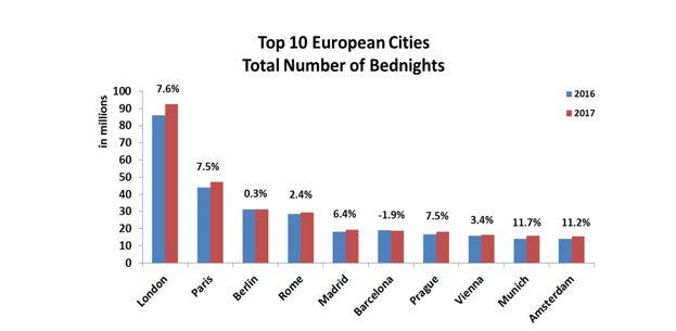
Claude / Journal of System and Management Sciences Vol. 10 (2020) No. 1, pp. 106-120

tourism is a growing industry, according to the Organization for Economic
Cooperation and Development (OECD) 2018, (Rödel E, 2017) It demonstrates that
the tourism industry is now responsible for 9% of the domestic product and
employment worldwide. Additionally, in the Netherlands, the travel industry is
developing (Rödel E, 2017).

 Fig. 1: Top 10 most visited European cities.

 Google has developed a tool called Google Trends that helps identify keywords
with the most search volume (Volcheck et al., 2018). In particular, search query
data provide valuable information about tourists’ intention, interests, and opinions.
Tourists use search engines and social media to obtain weather and traffic
information and to plan their routes by searching for hotels, attractions, travel
guides, and other tourists’ opinions. We use search query because when a tourist
interacts with the Internet through a search engine, a website, or a social media
platform, the traces of the interaction can be captured, stored, and analyzed (Paper,
2016).
 This study aims to investigate the opportunity to predict the number of visits
based on online tourist search. What people write on their microblogs reflects their
intent and desire relating to most of their common day interests (Length, 2016).
Taking this as strong evidence, we hypothesize that search queries of the person can
also be treated as a source of strong indicator signals for predicting their places of
visits, predict related with the three info highlights which are the date, tourists
number and locations those are from Google Trends dataset, the yield the mark is
number of Tourists in Amsterdam. From May 29th, 2016 up 31st December,2018
aggregate of 265,307 searchers from five nations (United Kingdom, Germany,
France, Belgium, Sweden), utilized with six predictive power search queries
(Amsterdam, Hotel Amsterdam, visit Amsterdam, travel Amsterdam, city trip
Amsterdam, Holiday Amsterdam) have been trained and tested by Hidden Markov
Model. The advantage of utilizing inquiry patterns to predict tourist data is two-fold.
First, query trends can utilize data up to the day before the forecast computation,
which could possibly be very significant in this setting because of the slacks in the

 107

Claude / Journal of System and Management Sciences Vol. 10 (2020) No. 1, pp. 106-120

distribution of the official measurement.

1.1. Tourist Journey
Before the tourist journey for the tourism sector is defined, it is important to
understand the general definition of tourist behavior. The process by which a tourist
chooses the place to visit or interests and opinions is defined as the tourist behavior
process (Song and Li, 2008; Dijkman and Ipeirotis, 2015; Nenonen et al., 2008).

 Fig. 2: Customer journey

 The city of Amsterdam publishes reports concerning the tourism industry branch
altogether on a yearly base. The reports concern trends in the tourism industry,
incoming tourism industry, Dutch tourism industry, the impact of the tourism
industry on the Dutch economy, employment opportunities in the branch and
diversion. In these reports, the city presents an information sheet about the previous
year and predicts the next year according to information from last year (Rödel,
2017).
 The reports give no understanding of the particular determining methods used to
structure these predictions (Li et al., 2017). However, there are some challenges
regarding the analysis, capture, search, sharing, storage, transfer, and visualization
and information privacy of big data, these challenges require new programs or
technologies to uncover hidden values (SMITH, 1946), Google Trends might be one
of those programs needed to enlarge the advantage of using big data to predict
tourism demand.
This has prompted the following research question for this study:
 1. What extent is the data provided by Google Trends useful for predicting night
passes in hotels in Amsterdam?
 To be able to answer this central research question the following sub-questions
will be answered:
 A. What predicting methods are utilized for predicting the travel industry
demands now?
 B. What is Google Trends and how does it work?
 C. Is Google Trends better predictor than the traditional forecasting method for
tourism in Amsterdam?

2. Literature review
This section reviews relevant studies in the areas of tourism demand and

 108

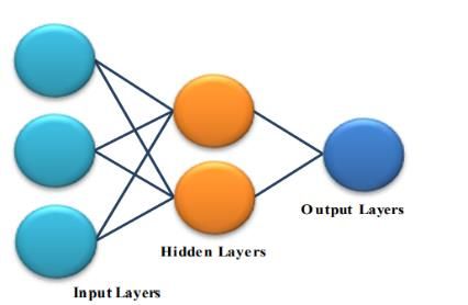
Claude / Journal of System and Management Sciences Vol. 10 (2020) No. 1, pp. 106-120

socioeconomic activity forecasting with search engine query data (Claveria and
Torra, 2014). Specifically, a few recent studies on forecasting tourism demand with
search engine data are also discussed. A decision making process in the travel
industry involves three following stages: information search, travel planning, and
trip arrangement of action (Cuhadar, 2014; Fesenmaier et al., 2016). The primary
goals of information search activities are to increase the overall quality of a future
trip and to decrease a perceived high risk, related to future travel.
 The development of ICTs and mobile computing devices have made the Internet
the main source of travel information. Search engines, such as Google and Baidu,
are the primary sources of tourism information, which shape tourist perceptions on
attraction image and encourage travel decisions.

2.1. Econometric models
Econometric models are models that attempt to replicate the important structures of
the real world (Song, 2010; Wijnhoven and Plant, 2017). These models can include
any number of simultaneous multiple regression analysis with several
interdependent variables. The major advantage of the econometric approach is the
ability to analyze causal relations. Basic utilized econometric models in the
literature are time-varying parameter (TVP) models, the vector autoregressive
(VAR) model and the Error correction model (ECM). About forecasting
performances; these models generally predict well although there remains more
research to be done to create significant improvements (Khadivi, 2016).

2.2. Artificial Neural Networks (ANN)
Artificial neural networks are forecasting methods that are based on simple
mathematical models of the brain (Wanjawa and Muchemi, 2014; Time, 2017; Jun
et al., 2018; Huang et al., 2005). A neural system comprises an input layer, an
output layer, and normally one or more hidden layers. Every one of these layers
contains nodes, and these nodes are connected to nodes at neighboring layer(s)
(Bursali, 1973). In Artificial neural networks, lagged values of the time series are
utilized as contributions to a neural network (like a direct autoregressive model).
We think about a feed-forward network with one hidden layer. The forecasts are
acquired by a linear combination of the information sources (Nath, 2005).

3. Methodology
This study aims for predicting the tourism industry demands, in the form of the
touristic night passes in hotels, with Google Trends data and CBS StatLine data
with the utilization of Hidden Markov Model HMM. The study takes the form of
time-series modeling since it depends on trends and patterns recognized by Google
trends. For that this advanced methodology will be utilized, in the first place, the
tourist journey theory is utilized to subtract search query terms. It will be researched

 109

Claude / Journal of System and Management Sciences Vol. 10 (2020) No. 1, pp. 106-120

how strong the relationship is between these terms and the pattern of specific
tourist’s statistics of the city of Amsterdam. Based on this, we attempt to discover
different search queries (keywords) for this field of interest. With this structure, the
distinction among clarifying and predicting will be made which leads us to the
following method questions:
 1. What are important keywords for predicting tourists in Amsterdam as indicated
by tourist journey theory?
 2. What are the important keywords for predicting tourists in a hotel in
Amsterdam according to Google Correlate?

3.1. The Workflow of our Method

 Fig. 3: The workflow of our method.

 This mechanism enables the users to interface the forecast procedure, which is
required feature from the training view. We propose to utilize Google Trends data
with HMM so that we can accomplish high prediction execution as well as acquire
great controllability to the tourism industry forecast. Concretely, we first set list of
keywords composed with ‘Hotel Amsterdam', Flight Amsterdam' 'Train to
Amsterdam’, 'City trip Amsterdam', Holiday Amsterdam’, 'Visit Amsterdam'
Tourist info Amsterdam and ' Amsterdam '. Second, we perform Granger Causality
Analysis (GCA) between tourism industry index and search query of Google Trends
to effectively figure out which search query has the most predictive power on the
index. Extensive experiments over real datasets demonstrate that our method not
only performs the traditional method, yet in addition gives controllability to the
tourism industry forecast.

 110

Claude / Journal of System and Management Sciences Vol. 10 (2020) No. 1, pp. 106-120

3.2. Data Collection
Data will be collected from Google Trends and the electronic database CBS
StatLine (2018). This study will focus on the calendar years 2016, 2017 and 2018.
The data set contains tourist’s arrival information for the Netherlands destination
are on a monthly level for a total period of thirty-six (36) months. As pointed out in
the hypothesis of this study, the search engine user needs to use keywords related to
the travel industry, get search query information and select fitting information.
 Table.1: Selected keywords and search engine users.

 The total number of search engine user for all keywords is 265,307, the keyword
has most search records is Amsterdam, have 53601 searches.

3.3. Hidden Markov Model
Hidden Markov Model is a predictable state mechanism which has some fixed
number of states. It provides a probabilistic framework for modeling a time series of
multivariate observations (Mathew et al., 2012; Daniel and Martin, 2018; Pai et al.,
2018)
 The advantages of HMM can be summarized as:
 1. HMM has a strong statistical foundation.
 2. It is able to handle new data robustly, computationally efficient to develop and
evaluate.
 For whatever remains of this research the following notations will be used with
respect to HMM:
 N= number of states in the model.
 M=number of distinct observation symbols per state.
 T= length of observation sequence.
 O=observation sequence
 transition matrix, where represents to the progress probability from
state to state .
 Observation emission matrix, where represent to the

 111

Claude / Journal of System and Management Sciences Vol. 10 (2020) No. 1, pp. 106-120

probability of observing . the prior probability, where represent to
the probability of being in state toward the start of the experiment, at time .
 the overall HMM model. As mentioned above the HMM is
described by and the and have the properties.
 and for all (1)

3.4. Artificial Neural Network (ANN)
ANN is a mathematical model or computational model based on biological neural
networks. It consists of an interconnected group of artificial neurons and processes
information using a connectionist approach to computation. He most important
neural network type is the Multi-Layer Perceptron (MLP) with the strict feed-
forward architecture of three layers. The connections between inputs and outputs
are typically made via one or more hidden layers of neurons or nodes. The input
layer is defined to assume the values of the input vector and does not perform any
additional computation, the hidden layer of neurons or nodes is fully connected to
the input and output layers and usually uses the sigmoid function as an output
function. Figure 3.3 shows a typical ANN with three inputs, and one hidden layer of
two neurons and one output (Polykalas et al., 2013).

 Fig. 4: Typical ANN with Three Inputs, One Hidden Layer of Two Neurons.

 The "generalized delta rule" is suggested by Rumelhart et al. and gives a recipe
for adjusting the weights on the internal units based on the error at the output. To be
more specific, let
 1
 E P =  J ( t pj - o pj)
 2
 (2)
 2
 Be the measure of the error in pattern p and let = ∑ be the overall measure
of the Error, where is the target output for the component of the actual output
pattern produced by the network representation with input pattern p. The network is
specified as
 o = f (net pj )
 pj j
 (3)

 112

Claude / Journal of System and Management Sciences Vol. 10 (2020) No. 1, pp. 106-120

3.5. Vector Auto-Regressıve (VAR)
The vector auto regression (VAR) model is one of the most successful, flexible, and
easy to use models for the analysis of multivariate time series. The VAR model is
useful for describing the dynamic behavior of financial time series and for
forecasting. There are many studies about modeling financial time series with VAR
models [7].

3.6. Hidden Markov Model as a solution
In this section we develop an HMM-based tool for time series forecasting, for
instance, to predict tourism demands, while implementing the HMM, the choice of
the model, choice of the number of states and observation symbol (continuous or
discrete or multi-mixture) become a hard task.
 Our observation here being constant as opposed to discrete, we choose
experimentally upwards of 3 mixtures for each state for the model destiny. For the
prior probability , a random number was chosen and normalized so that
 .
 The dataset being continuous, the probability of emitting symbols from a state
cannot be calculated. Therefore, a three-dimensional Gaussian distribution was
initially chosen as the observation probability destiny function. Thus we have
 b j (o j ) =  c jmn [o,  jm u jm ]1  j  N (4)

 =vector of observations being demonstrated.
 = mixture coeff. for the m-th mixture in state j, where
 = mean vector for the m-th blend segment in state j.
 ℵ= Gaussian density.
 For training the model, three years (2016, 2017, 2018) Google Trends data and
information from CBS StatLine were utilized and recent last one year's data were
utilized to test the efficiency of the model.

3.6.1. Keywords Extraction and Evaluation
In this section, we extract and evaluate Google Trends keyword. Our aim is
predicting tourist number in Amsterdam, so we focus on analyzing the keywords in
general. First, we evaluate the predictive power of different keywords via GCA and
determine the most predictive Keywords. Because of the massive amount of
keyword records, we used a CPA to reduce them. The filter method removes
keywords containing contain zero records and keeps keywords containing records.
 Formally, the following two equations hold:
 lag
 yt = yo +  yiYt −i +  t (5)
 i =1

 lag lag
 yt = yo +  yiYt −i +  xi X t −i +  t (6)
 i =1 i =1

 113

Claude / Journal of System and Management Sciences Vol. 10 (2020) No. 1, pp. 106-120

 Above, and are time variables (month), and lag is the upper bound of lagged
months. We perform GCA the growth of the tourism industry volume record (Y)
and keyword (X). We determine the keyword that has the most predictive power
and its corresponding lagged value as according to the following two rules:
 1. Find which is at a statistically significant level ( pvalue  0.1) .
 2. Find which reduces significantly comparing to its precursor (distinction  0.25).
Definition 1: Given an observation sequence O = o1, o2, ..., oT (showing
historical tourists from CBS StatLine), a relative label sequence L = l1, l2, ..., lT
(demonstrating next month tourists number) and an HMM λ, the state label pi
denotes the most probable label that state q i should have. Formally, above,
 yti = p(st = qi \ o,  ) means the probability that the HMM λ stays at state q i at the
time, which can be processed by the forward-backward technique.
Definition 2: Given an observation sequence O = o1, o2, ..., oT and an HMM λ,
the experimental visit rate indicates the part of the time that the HMM λ spends at
state q i i.e .
 1 T
 vi =  yti
 T t =1
 (7)

Definition 3: Given an observation sequence O = o1, o2, ..., oT , a relative label
sequence, L = l1, l2, ..., lT and an HMM λ, the exact state risk ri indicates the
rate of erroneous visits to state q i Formally,
 1 T
  t =1,lt  pi yti (8)
 ri = T
 vi

3.6.2. Hidden Markov Model Training
Given a coverage bound , numerous observation sequences and a label
 q
sequence L, we train an HMM and recursively refine the heavy state h until there
is no heavy state remaining. The training process comprises of the following
progress:
 1. Initialize the root HMM  0 with random parameters, and train it with the set
 of historical tourists from CBS StatLine and Google trends information. The
training algorithm is Baum-Welch variation adjusted observation sequences.
 2. Compute state label p i , empirical visit rate v i and empirical state risk for
each state qi in the root HMM λ0. Under the coverage bound , compute the reject
subset RS of the root HMM  0 to identify which state is the heavy state q h . If
there is no heavy state, then the training is done.
 3. Initialize a random HMM  random to replace the heavy state q h , so a
refined HMM  refine is obtained. Train the refined HMM  refine with the
previous set of multiple observation sequences until it converges.

 114

Claude / Journal of System and Management Sciences Vol. 10 (2020) No. 1, pp. 106-120

 1
  (y1j (i) +  t =i−11  k =1,k  h  t,k, j(i) )
 K T N
 i =1 (9)
 pi
 j =
 Z
 1
    t ,k , j (i )
 K Ti−1
 i =1 t =1
 pi
 a jk =
 1
    (10)
 N +n
  t , k ,l ( i )
 k Ti −1
 l = N +1 i =1 t =1
 Pi
 1
  
 k Ti
 i =1 t =1,ot( i ) =um
 ytj(i )
 pi
 b jm = (11)
 1
  i=1 p  t =1 ytj(i )
 k Ti

 i

 Above, Z is thestandardization factor of j ,
and ( t, j,k = Ps t = q j , s t + 1 = q k | O,  ) ) is the probability of HMM  from state
q j to state q k time, which can be efficiently computed by the forward-backward
procedure.
 4. Compute exact visit rate vi and experimental state risk ri for each state qi in the
refined HMM  refine. Under the coverage bound , compute the reject
 RS subset of the refined HM  refine to recognize which state is the
overwhelming state q h . If there is a heavy state, go to Step 3.

3.6.3. Hidden Markov Model Prediction
Given a trained stream HMM and another observation sequence
O = o1,o2,...,oT , e forecast the last label lT in the relative label sequence L as
indicated by O through recursively finding the most l probable state q most t. The
prediction procedure comprises the following steps:
 1. Find the most probable state q most at the last time T by the computing  Ti of
all states in the root HMM λ0.
 2. If q most is a refined state q refined , reset the most probable state q most by the
computing  Ti of new states added to the following dimension refined HMM 
refine, and go to Stage 2.
 3. If q most is in the reject subset RS , no forecast is made; something else, the
label p most of the state q most is yield as the prediction result of the last label p most
in the relative according to O .

4. Conclusion and Proposals
In this section, we present experimental evaluation results. First, we introduce an
experimental datasets and computing environment. Then, we present and analyze
the results of the GCA. Finally, we compare our method and two existing methods
to demonstrate the advantage of our method.

 115

Claude / Journal of System and Management Sciences Vol. 10 (2020) No. 1, pp. 106-120

4.1. Statistics of Extracted Keywords
We extract keywords from Google Trends and keep the extracted more data using
different keywords in monthly periods as long have not enough data. Then we get
six predictive power keywords. The results of those keywords plotted here.

 Fig. 5: Keyword “Amsterdam”.

 Fig. 6: Keyword “Visit Amsterdam”

4.2. Results of Granger Causality Analysis
After effects of Granger Causality Examination, we perform GCA on the extracted
and analyze Google Trends data. We treat the Google Trends data volume as time
series respectively, while taking every keyword as time series. The range is set
from 1 to 3.We present the pvalue results of Google Trends information in Table
4.1.By checking the outcomes in the table, we select three months ( i.e., lag=3 )

 116

Claude / Journal of System and Management Sciences Vol. 10 (2020) No. 1, pp. 106-120

lagged Amsterdam(Am). We use Google Trends keywords as the predictive pointer
of the travel industry requests because of following two reasons:
 1. Most under three months of lagged Amst. Google Trends keywords achieve a
significant level (  0.1) , and its value is 0.061.
 2. All pvalue under three months of lagged Amst. Google Trends search query
(keywords) decrease significantly (difference 0.25) comparing to pvalue under
two months lagged Amst, Google trends keyword.
 Table 2: pvalue Results of Google Trend keywords (allpvalue*  0.1)
 Lag Google Trends
 Keywords Amst Hotel Am Visit Am Travel Am City trip Am Holiday Am
 1 0.407 0.266 0.651 0.686 0.525 0.250
 2 0.467 0.436 0.638 0.548 0.702 0.315
 3 0.061 0.150 0.656 0.276 0.731 0.328

4.3. Prediction Performance Comparison
We compare our method and two existing methods, in which two methods exploit
Google trends. These two methods and our method all incorporate 3months lagged
Am. Our method performs well on Google trends to predict the tourist industry
demands. The two methods are:
 1. The Vector Autoregressive (VAR) framework treats tourism information and
Google Trends as a coordinated vector to make prediction based linear regression.
 2. Artificial Neural Network (ANN) utilizes two nodes of "big" and "small" as
yield layer and puts the two tourist’s information and Google Trends to include a
layer to make the prediction. Well as our method is the best model for predicting the
tourism industry demands utilizing search engines with controllability.
 Table 3: Comparison with two methods using Google Trends.
 MODEL ERROR R ATE (%)
 VAR 28.132
 ANN 33.667
 HMM 24.109

 Correlation with existing strategies utilizing Google patterns, as HMM’s
performance is flexible by the coverage bound CB , we set 3 values between 1.0
and 0.1 for CB to evaluate HMM. A smaller CB value means that HMM puts
more restriction on prediction output, which prompts a smaller error rate. For the
two existing methods, we tune their parameters to get the best results.
 All experimental results are presented in Table.3; we can see that among the two
existing methods, VAR has the smallest error rates 28.132 %. For the three cases,

 117

Claude / Journal of System and Management Sciences Vol. 10 (2020) No. 1, pp. 106-120

by CB 's an incentive respectively, HMM can get smaller error rates 24.109 %
than the two existing methods. Also, with CB =0.1 HMM achieves the lowest error
rate on all two of datasets. All the more significantly, the error rate of HMM is
controllable, while the existing methods do not have such a feature. The results of
predicting tourism demands in Amsterdam using Google Trends is plotted here.

 Fig. 7: Result of Predict Tourism demands in Amsterdam.

5. Conclusions
We proposed to use Google Trends forecast based on HMM. First, we used six
predictive power keywords, at that point we performed GCA between over massive
keywords to figure out which Google Trends keywords has the most predictive
power on tourism forecast. Finally, we extended method with three months lagged
Amsterdam (Amst) Google Trends data not only performs better than existing
methods, yet additionally gives a controllability mechanism to the tourist industry
prediction.

6. Acknowledgments
This research is part of my master’s thesis. I thank my master tutor prof. Jitao sang
and I thank for Dalin Zhang for his warm help.

References
Bursali S (1973). Determination of the Minimum Number of Samples for the
Compaction Control of Impervious Fills. Tour. Manag. 70 1-15

 118

Claude / Journal of System and Management Sciences Vol. 10 (2020) No. 1, pp. 106-120

Claveria O and Torra S (2014). Forecasting tourism demand to Catalonia: Neural
networks vs. time series models Econ. Model. 36 220-8

Cuhadar M (2014). Modelling and Forecasting Inbound Tourism Demand to
Istanbul: A Comparative Analysis Eur. J. Bus. Soc. Sci. 2 101-19

Daniel J and Martin J H (2018). Hidden Markov Models Speech Lang. Process. 1–
17

Dijkman R and Ipeirotis P (2015). Using Twitter to predict sales: a case study ar
Xiv Prepr. arXiv 1503.04599. 471, 1-14

Fesenmaier D R, Pan B and Xiang Z (2016). Destination Competitiveness and
Search Engine Marketing

Huang Y, B S Z, Huang K and Guan J (2005). Database Systems for Advanced
Applications 3453 435-51

Jun S P, Yoo H S and Choi S (2018). Ten years of research change using Google
Trends: From the perspective of big data utilizations and applications Technol.
Forecast. Soc. Change, 130, 69-87

Khadivi P, Tech V and Tech V (2016). Wikipedia in the Tourism Industry :
Forecasting Demand and Modeling Usage Behavior Proc. 30th Conf. Artif. Intell.
(AAAI 2016) 4016-21

Length F (2016). Tourism forecasting by search engine data with noise-processing.
10 114-30

Li X, Pan B, Law R and Huang X (2017). Forecasting tourism demand with
composite search index. Tour. Manag. 59 57-66

Mathew W, Raposo R and Martins B (2012). Predicting future locations with
hidden Markov models UbiComp’12 - Proc. 2012 ACM Conf. Ubiquitous Comput.
911-8

Nath B (2005). Stock Market Forecasting Using Hidden Markov Model : A New
Approach

Nenonen S, Rasila H and Junnonen J M (2008). Customer Journey – a method to
investigate user experience W111 Res. Rep. Usability Work. Phase, 2, 54-63

 119

Claude / Journal of System and Management Sciences Vol. 10 (2020) No. 1, pp. 106-120

Pai P F, Hong L C and Lin K P (2018). Using Internet Search Trends and Historical
Trading Data for Predicting Stock Markets by the Least Squares Support Vector
Regression Model Comput. Intell. Neurosci. 2018

Paper W (2016). Forecasting travelers in Spain with Google queries Máximo
Camacho and Matías Pacce

Polykalas S E, Prezerakos G N and Konidaris A (2013). An algorithm based on
Google Trends’ data for future prediction. Case study: German elections IEEE Int.
Symp. Signal Process. Inf. Technol. IEEE ISSPIT , 69-73

Rödel E (2017). Forecasting tourism demand in Amsterdam with Google Trends 1-
70

SMITH S W (1946). The hypopietic patient. Practitioner,156, 381-3

Song H and Li G (2008). Tourism demand modelling and forecasting-A review of
recent research. Tour. Manag. 29 203–20

Song H (2010). Tourism Forecasting : Accuracy of Alternative Econometric Models
Revisited Symp. A Q. J. Mod. Foreign Lit.

Time B T (2017). Fw : [ TELKOMNIKA ] # 5993 : Foreign Tourist Arrivals
Forecasting Using Recurrent Neural Network Backpropagation Through Time To :
Oger Vihikan

Volcheck E, Song H, Law R and Buhalis D (2018). Forecasting London Museum
Visitors Using Google Trends Data e-Review. Tour. Res. 4

Wanjawa B W and Muchemi L (2014). ANN Model to Predict Stock Prices at Stock
Exchange Markets 1–23

Wijnhoven F and Plant O (2017). Sentiment Analysis and Google Trends Data for
Predicting. Car Sales ICIS. Proc. 1–16

Yang X, Pan B, Evans J A and Lv B (2015). Forecasting Chinese tourist volume
with search engine data. Tour. Manag. 46, 386–97

Yang Y, Pan B and Song H (2014). Predicting Hotel Demand Using Destination
Marketing Organization’s Web Traffic Data J. Travel Res., 53, 433–47

 120