Prediction of feed-in power from photovoltaics in local distribution networks - DGPF
←
→
Page content transcription
If your browser does not render page correctly, please read the page content below
38. Wissenschaftlich-Technische Jahrestagung der DGPF und PFGK18 Tagung in München – Publikationen der DGPF, Band 27, 2018

               Prediction of feed-in power from photovoltaics
                        in local distribution networks

                MOSTAFA ELFOULY1, ANDREAS DONAUBAUER1 & THOMAS H. KOLBE1

        Abstract: Due to the shift of power production from highly centralised power plants to de-
        centralised power production with renewable energy, the role of local distribution networks
        has changed. Originally, these networks were designed to distribute electric power from a
        centralised source to consumers. However, nowadays, the increasing number of climate-
        dependent decentralised energy production systems connected to local distribution networks,
        such as photovoltaics, affect the network stability. Thus, network operators need decision
        support methodology in order to cope with the network uncertainty. As a central part of the
        decision support system, climate-dependent forecast for feed-in power is required with high
        spatial resolution. In this paper, a method for the prediction of feed-in power production
        from photovoltaics, based on georeferenced power production and meteorological data is in-
        troduced.

1 Introduction
For decades, centralised power plants have been the operating model for electricity generation
across Europe. This means, that huge quantities of electricity are being generated by power
plants, that are physically clustered in a specific area or region located far away from the con-
sumer (GREEN & SONNREICH 2014). The electricity being generated by the centralised power
plants is being distributed through the electric power grid to multiple users (ACKERMANN et al.
2001).
Based on the Department of Economic and Scientific Policy within the EU parliament in June
2010, there has been a paradigm shift from centralised power plants to a more decentralised en-
ergy system. This shifts the narrative from passive to active consumers, in the sense that they can
act as power producers as well (ALTMANN et al. 2010; COSSENT et al. 2009). End consumers, in
turn, are often installing solar panels to cover their power needs and the excessive power are to
be fed-in to the grid (CARLEY 2009). However, these climate-dependent decentralised energy
production systems affect network stability. Hence, network operators need decision support
tools for coping with network instabilities.
In this contribution, a method for feed-in power prediction from photovoltaics, based on georef-
erenced power production and climate data is described. The method takes into account that pho-
tovoltaic power production is influenced by various parameters: a) geographical location on earth
and orientation of the panels, b) time of the year (changing sun elevation over the year), c) time
of the day (HOSTE et al. 2009) (changing sun position over each day), d) climate (e.g. weather,
wind, cloud, atmospheric conditions, etc.), e) shadowing effects caused by local topography
(SALVATORE & FRANCISCO 2015), and f) panel-specific parameters (e.g. efficiency of the solar

1
    Technische Universität München, Lehrstuhl für Geoinformatik, Arcisstr. 21, 80333 München,
    E-Mail: [mostafa.elfouly, andreas.donaubauer]@tum.de

                                                             199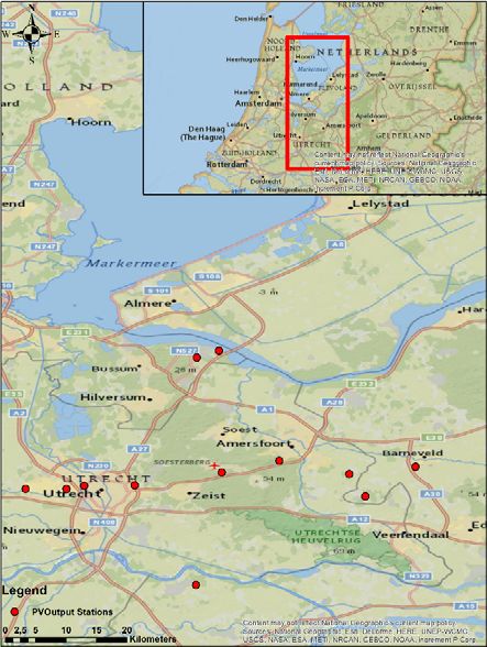
M. Elfouly, A. Donaubauer & T. H. Kolbe

panel, condition like dust, dirt or snow cover). Whereas, the aforementioned parameters (a-e) do
play a pivotal role in the global horizontal irradiance (GHI), diffuse horizontal irradiance (DHI),
and shortwave radiation received on the Earth surface, the panel-specific parameters are highly
individual.
Within the course of this research, diverse meteorological aspects that play a role in the feed-in
power have been investigated. As part of a state-of-the-art analysis, two approaches to compute
or predict the feed-in power from photovoltaics have been identified: An analytical approach and
an observation-based one.

2 Related Work
The amount of solar irradiation that reaches the surface of the solar panels determines how much
power can be produced by a specific solar panel. Additionally, the panel-specific parameters (see
section 1) contribute to the amount of power being produced and fed into the network. In this
contribution, we have identified two approaches for tackling the issue of predicting the feed-in
power from photovoltaics: an analytical approach and an observation-based approach.

2.1 Analytical Modelling
In the analytical approach, each and every aspect that plays a role in the computation of the
amount of power being generated by the solar panel is to be thoroughly studied and a computa-
tional formula is to be obtained. As earlier mentioned, there are a variety of factors that do influ-
ence the feed-in power from photovoltaics.
One of the areas that have been studied in depth was the cloud coverage and its impact on the
solar irradiation. In a research study by LUMB (1963) founded on a former study by KIMBALL
(1928), an empirical correlation function between the average daily short-wave radiation and the
fraction of sky covered by cloud has been introduced. However, that empirical formula that has
been introduced did not take into account the different types of clouds. LUMB (1963) comple-
ments KIMBALL’S (1928) work by classifying and identifying different types of clouds. In his
study, clouds were divided into nine categories, mainly based on their intensity (amount of
cloud) and altitude. In addition to that, scattering of solar irradiation also varies based on, the
cloud optical depth, cloud geometry, and the direction of the incident solar radiation (MCKEE &
COX 1974; AIDA 1977).
However, the data required for these computations are typically not available, which makes it not
practical in deducing a computational formula for estimating the short-wave radiation that is re-
ceived at the solar panel. Also, due to the diversity of the domains that ought to be covered to
precisely compute the amount of feed-in power from photovoltaics, an analytical model consid-
ering all the aforementioned factors would be very complex. Furthermore, from a practical point
of view, the panel-specific parameters (see section 1) cannot be obtained for individual house-
holds. Hence, the second approach, which seems to be more applicable and more examined re-
cently, is the observation-based approach.

                                                200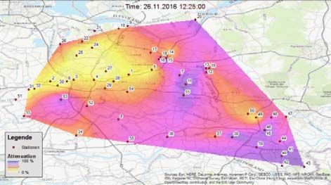
38. Wissenschaftlich-Technische Jahrestagung der DGPF und PFGK18 Tagung in München – Publikationen der DGPF, Band 27, 2018

2.2 Observation-based Modelling
In contrast to analytical modelling, observation-based approaches rely on correlating the obser-
vations of different phenomena with each other using statistical methods. In a study by YUAN et
al. (2015), a correlation between the normalised solar radiation difference and the cloud optical
thickness was built. An exponential correlation between the amount of solar radiation increase
and the cloud optical thickness decrease was observed. In another research work by YANG et al.
(2012), a forecast analysis between the Global Horizontal Irradiance (GHI) and Direct Normal
Irradiance (DNI) based on a cloud cover index was developed. These studies rely on an observa-
tion-based approach to detect the correlation between cloud coverage and solar irradiation using
NASA MODIS data (PLATNICK et al. 2015).
By taking into account these research studies, we concluded that an observation-based approach
does overcome individual missing or prone to error parameters, as of the case in the analytical
one. Additionally, various meteorological parameters can be correlated to the solar irradiation.
This, in turn, allows for studying certain meteorological phenomena and their direct or indirect
impact on the photovoltaic power generation (JEREZ et al. 2015).
As a result, it has been decided that we further investigate the observation-based approach in
order to predict the power output from photovoltaic cells under certain weather conditions.
However, the studies mentioned above do not take into account local topography and panel-
specific parameters (see section 1), which are important for predicting the feed-in power in local
distribution networks, but which are not obtainable in most cases. In our research we propose an
observation-based approach, which tries to overcome these problems.

3 Proposed Observation-based Approach
Our approach relies on statistical analysis of georeferenced historic power production measure-
ments from photovoltaic systems installed in local distribution networks and georeferenced his-
toric meteorological data. Figure 1 gives an overview of our approach. The numbers shown in
the Figure correspond to the numbering of the sections in this paper.

3.1 Acquisition of power production data from photovoltaics stations
The first step in this research project was to obtain a reliable and continuous stream of photovol-
taic power production data. Online services for providing crowd sourced photovoltaic power
data, such as PVOutput2 were inspected and analysed. More than 50 photovoltaic stations in the
area of Utrecht (Netherlands) were picked from PVOutput and selected for further investigation
(see Figure 2). Power production data acquisition was limited to a period of 12 months back,
because of PVOutput limitations. However, although PVOutput provides free online service for
photovoltaic output data, it does not guarantee their consistency or sustainability.
In order to take the observation-based approach a step further and correlate power production to
meteo-rological factors, a con-tinuous stream of power readings was essential.

2
    http://www.pvoutput.org

                                                             201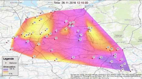
M. Elfouly, A. Donaubauer & T. H. Kolbe
Fig. 1. Overview of the proposed approach
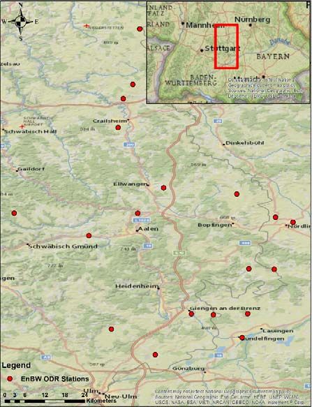
Therefore, the German energy company EnBW ODR provided us with photovoltaic power pro-
duction data for 22 stations (spatial distribution see Figure 3) over the course of 13 months with
15 minutes temporal resolution. The same workflow has been applied on the EnBW ODR and
the PVOutput data and the readings have been geo-referenced and stored in a geo-database in
order to allow for spatial analysis, such as spatial autocorrelation of the power production data,
spatial interpolation, and spatial correlation with meteorological data (see 3.5). In the following
sections, the further steps of our approach are described. The outcomes are illustrated using ei-
ther the crowd sourced PVOutput data or the data provided by the energy company EnBW ODR.
3.2 Maximum Power Estimation for each Station
In order to overcome the individual panel specific characteristics, we needed to derive a parame-
ter, which accounts for all the influences and makes different photovoltaic systems comparable.
Hence, we needed to identify the maximum expectable power that can be generated by a specific
station at a particular point in time on a particular day. The maximum generated power varies on
daily basis, because of the factors, such as change of inclination of the sun during the year (shad-
owing situation), and season specific atmospheric conditions. Therefore, we had to create the
maximum power curve for each individual day of the year. In order to measure the maximum
power at each point in time produced by a certain solar panel, we resorted to historic measure-
ments. The maximum power produced for a specific station was computed for each day of the
202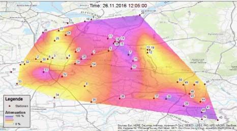
38. Wissenschaftlich-Technische Jahrestagung der DGPF und PFGK18 Tagung in München – Publikationen der DGPF, Band 27, 2018

year applying a moving window approach as follows: for each day of the year, for every 15
minutes time step, the generated power is compared to its relevant time values for +/-15 days,
then the maximum reading is being selected (see Figure 4). The period of +/-15 days was chosen,
because we assumed, that within this period the probability is high to find clear sky conditions.
The maximum generated power was then assumed to be the maximum expected power that can
be obtained from a particular solar panel under clear sky conditions at this point in time.

Fig. 2: PVOutput stations                                              Fig. 3: EnBW ODR stations

   P
                                                                                           Pmax for 8:00 AM
                                                                                              on April 4
                          We are interested in Pmax for
                              8:00 AM on April 4

                                                                                                                                t
          April 2 2016,            April 3 2016,     April 4 2016,         April 5 2016,        April 6 2016,   April 7 2016,
            8:00 AM                  8:00 AM           8:00 AM               8:00 AM              8:00 AM         8:00 AM

Fig. 4:      Moving window approach for maximum power computation

                                                                     203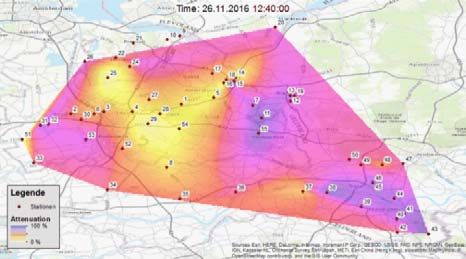
M. Elfouly, A. Donaubauer & T. H. Kolbe

3.3 Attenuation Computation and Spatial Interpolation
Considering the fact that various meteorological conditions may reduce the amount of power
being generated by a certain percentage and by learning the maximum expected power produc-
tion for each station at a specific point in time (see section above), we derived a specific attenua-
tion function for each station along the year. Attenuation is defined as the percentage of power
being lost, due to meteorological conditions. An attenuation value of 0% means that a specific
station generates the maximum expectable energy for this point of day and time, taking into ac-
count the station-specific non-meteorological factors, such as date and time, efficiency, panel-
condition and local topography. An attenuation value of 100% means that this station produces
no power at all. In order to determine the current attenuation percentage, a ratio between the
measured and maximum expectable power at a specific point in time has to be built. The attenua-
tion accounts for all the influences and the afore-mentioned parameters – apart from meteorolog-
ical factors - and therefore makes different stations comparable:

                   Attenuation   %   1    ∗ 100

where P is the measured power at a specific point in time and Pmax is the maximum expectable
power at this point in time under clear sky conditions (see 3.2).
Then, we generated daily-based, seasonal-based, and station-based, diagrams for plotting the
actual power that is being produced by a specific station, maximum power at each point in time,
and the attenuation percentage (see Figure 5).
Then, three scenarios have been considered, in order to observe various correlation aspects. The
first one is to indicate the meteorological influence, such as cloud coverage and its impact on the
power production. Thus, we decided on two consecutive dates where one is cloudy and the other
one has clear sky conditions (see Figure 5). It can be noted, that there is severe power drop on
                                                                           the cloudy day, com-
                  100

                                                                           pared to the clear sky
                                                                           day. However, there
                  80

                                                                           might have been other
                                                                           meteorological factors
 Percentage [%]

                                                                           that have played a role
                  60

                                                                           also. In the second sce-
                                                                           nario, we checked for
                  40

                                                                           spatial auto-correlation
                                                                           between nearby sta-
                  20

                                                                           tions, in order to ob-
                                                                           serve for certain mete-
                                                                           orological phenomena,
                  0

           6      8       10    12       14       16       18    20     22 such as cloud move-
                               Hours of the day [hh]                       ment, that occur over a
Fig. 5: An example for actual power production, maximum power, and         certain region (see Fig-
                                                             nd
          attenuation percentage for Pasij station on April 2 2016. Ex-    ure 6). It can be noticed
          ample using PVOutput                                             that the power curve is

                                                204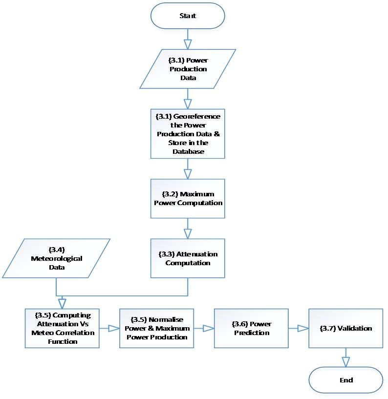
38. Wissenschaftlich-Technische Jahrestagung der DGPF und PFGK18 Tagung in München – Publikationen der DGPF, Band 27, 2018

almost the same for both nearby stations, because they do get exposed to similar conditions at
this point in time. The last scenario was studying the seasonal effect and its correlation to the
amount of power that can be produced by a certain station (see Figure 7). In that last scenario
(see Figure 8), we can study seasonal effects of photovoltaic power production.
        Percentage [%]

                                                                                  Percentage [%]
                               Time (seconds till midnight)                                             Time (second till midnight)
    Percentage [%]

                                                                                    Percentage [%]

                               Time (seconds till midnight)                                               Time (second till midnight)

 Fig. 6:                 Clear Sky vs Cloud for Moorstenweg                       Fig. 7:            Spatial auto-correlation on Fregatstraat &
                         station on 9th and 10th of May consecu-                                     Moorsterweg on March 17th 2016 consec-
                         tively – examples using PVOutput data.                                      utively using PVOutput data. The green
                         The green curves differ substantially.                                      curves have nearly the same shape.
   Legend
                                                              Percentage [%]

                          Normalised actual power
                         Smoothed normalised maximum power
                         Smoothed attenuation percentage

                                                                                                       Time (second till midnight)
                                                               Percentage [%]

 Fig. 8:                 Seasonal effect for Fregatstraat
                         station on January 25th and July
                         18th 2016 consecutively using
                         PVOutput data
                                                                                                       Time (second till midnight)

                                                                                205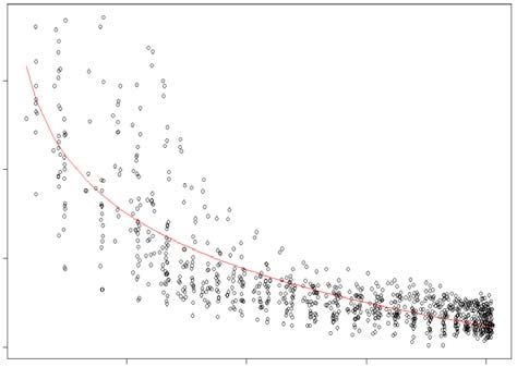
M. Elfouly, A. Donaubauer & T. H. Kolbe

Afterwards, a spatial interpolation between the stations has been performed, in order to deduce
attenuation fields, which show spatial distribution and the change of attenuation throughout the
day, month, and year for the whole area of study (see Figure 9). The spatial interpolation was
carried out using the natural neighbours interpolation algorithm (SIBSON 1981), because of it
creates a smooth field, whereas the observations at the known data points are preserved.

Fig. 9:   Attenuation field of four consecutive points in time in the Utrecht area: Top left 12:05 pm, top
          right: 12:15 pm, bottom left: 12:25 pm, bottom right: 12:40 pm. Data source: PVOutput

The attenuation field now allows to predict the feed-in power for a station installed at an arbi-
trary location within the extent of the field and for a specific point in time. This use case is relat-
ed to a real-world problem, that energy companies face. Whereas, only few stations have smart
meters installed, the energy companies need to predict feed-in power for all stations connected to
their network. Thus, the attenuation field can be used to predict the potentiality of power produc-
tion for stations with no smart meters installed, by extracting the attenuation values for the geo-
graphic locations of the power stations from the field. The amount of power to be produced is
then to be computed from the extracted attenuation values. In order to do so, the maximum pow-
er that is ought to be generated from this particular panel still has to be known.

3.4 Meteorological Data Acquisition
Acquiring meteorological data for the same spatial region as of the photovoltaics stations is cru-
cial. Also, the time span and temporal reference system for the various meteorological attributes
has to match with that of the power production readings. Hence, within the scope of this project,
we obtained satellite-based meteorological data for our test region with a spatial resolution of

                                                    206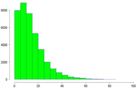
38. Wissenschaftlich-Technische Jahrestagung der DGPF und PFGK18 Tagung in München – Publikationen der DGPF, Band 27, 2018

3x3km and a temporal resolution of 15 minutes from the company METEOBLUE3. The obtained
data varied from cloud coverage and temperature to Global Horizontal Irradiance (GHI) and Dif-
fuse Horizontal Irradiance (DIF). In order to prepare for correlation with power production data,
the meteorological data had to be geo-referenced. Then, as a last step before correlating the me-
teorological readings with the power production readings, both of those readings had to be trans-
formed to the same time base (UTC offset of one hour was chosen).

3.5 Finding a correlation function
By analysing the historic observations and meteorological data, a correlation function between
the attenuation and the various meteorological factors derived from satellite observations, such
as cloud cover and solar irradiance could be determined. The derived correlation function, allows
to predict the attenuation field for a specific future point in time from weather forecast.
As a first step of the correlation process, geo-location and date-time of the power production,
attenuation and meteorological data were used for joining the readings in a common database
table. Then, scatter plots were produced to examine for potential correlation. It is to mention, that
night time was excluded from our study, since it gives us a false indicator of strong correlation
where readings from power production as well as solar irradiation are zero.
                                   80000
                                    60000
                       Power (W)
                                   20000 40000

                                                 100   200   300    400    500   600     700      800
                                                                   GHI (W/m2)

Fig. 10: Scatter plot between GHI & power for Spraitbach station in August 24th 2016. Data source:
         Power production: EnBW ODR; Meteorological data: Meteoblue

By analysing Figure 10, a mostly linear correlation between the GHI (W/m2) and the produced
power (W) for a specific station can be observed. A linear regression function was then generat-
ed and checked thoroughly. In addition to that, we inspected the correlation between the attenua-
tion and GHI. However, a linear regression in that case was not the best fit (see Figure 11). Thus,
we generated a polynomial regression function of the 5th degree to correlate GHI with the attenu-
ation percentage.

3
    https://content.meteoblue.com/

                                                                    207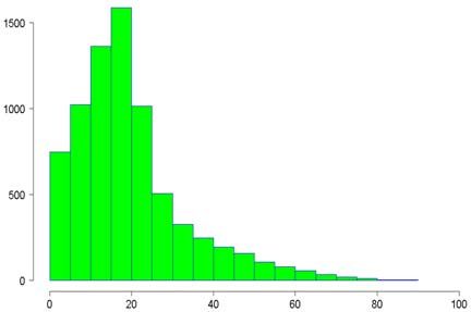
M. Elfouly, A. Donaubauer & T. H. Kolbe

                                      60
                    Attenuation [%]

                                      40
                                      20
                                      0

                                           200         400        600          800
                                                   GHI [W/m2]
Fig. 11: Scatter plot between GHI & attenuation for all the stations on September 24th 2016. Data
         source: Power production data: EnBW ODR; Meteorological data: Meteoblue

By examining the correlation for longer periods of time, we concluded that there is a higher cor-
relation between the GHI and the attenuation, than between the GHI and the power production,
specifically under non-clear-sky-conditions. Hence, as a last step before forecasting, we extended
our correlation over a 12-months timespan to assess the goodness of fit of the model. Further-
more, we studied the correlation separately for each season, in order to evaluate the fitting model
and determine if the correlation varies from season to season.
As a result, of that, the goodness of the fitting model across the whole year is estimated to be
0.74 R squared. The fitting model operates during autumn with 0.85 R squared and the least dur-
ing summer with 0.63 R squared. Additionally, it was found out that by taking into account 12
months of historical data, a linear regression equation could be deduced, which is in contrast to
the results when we take only small sample data as seen in Figure 11.
We plotted the diverse meteo-rological aspects that we have obtained, such as cloud coverage
and temperature against the attenuation to examine if there is a noticeable correlation between
them (see Figure 11). However, temperature did not play a significant role in the amount of pow-
er being generated. As for cloud coverage, while it plays a role in the amount of solar radiation
received on the earth surface, as we explained in the introduction, there was no direct correlation
between the power production and the cloud coverage. This is because, in the meteorological
data available, cloud coverage is expressed as a percentage representing the fraction of a 3×3
kilometres tile covered by clouds with 15 minutes temporal resolution. This means, that clouds
can be formed within this time period without being detected. Also, different formations of
clouds react to solar radiation differently as earlier discussed in section 2.2, and cannot be dis-
criminated in the meteorological data available. Based on the regression model that has been
generated in section 3.5 and by feeding GHI as input to the model, we could predict the attenua-
tion percentage on that particular day. As demonstrated in Figure 13, the blue line in the middle
is the estimated fitting line, while the red and the green ones are the lower and upper boundaries
consecutively of the 95% confidence interval. Thus, the correlation function enables us to predict
the attenuation field for a specific future point in time from weather predictions. Moreover, it
allows us to predict the feed-in power for a specific station and for a specific future point in time
from the predicted attenuation field, by reversing the attenuation formula:

                                                 208
38. Wissenschaftlich-Technische Jahrestagung der DGPF und PFGK18 Tagung in München – Publikationen der DGPF, Band 27, 2018
Attenuation percentage [%]
1000
60
800
Power [W]
600
40
400
200
20
3 8 13 18 23
0
Coordinated Universal Time [hours] 200 400 600 800
GHI [W/m2]
Fig. 12: Meteorological factors vs photovoltaics Fig. 13: Estimated attenuation percentage for
power production for a clear sky day for Al- Schrozberg on July 11th 2016. Data
theim (Alb) on September 14th 2016. Data source: Power production: EnBW ODR;
source: Power production data: EnBW Meteorological data: Meteoblue
ODR; Meteorological data: Meteoblue
%
Power 1 ∗
Validation
In order to evaluate the estimation, we divided our data into training data and test data. By taking
into account the seasonal influences, we used training data from different seasons, in order to be
able to have a proper estimation. Validation in our approach went through different steps. In a
first step the acquired data was validated. In order to determine if the power production and me-
teorological data are in the same time zone, we generated diagrams for various meteorological
factors against power (see Figure 12). It can be clearly observed that the power production (W)
and the clear sky shortwave (W/m2) do overlap and there is no time lag. Also, it can be clearly
observed that the given day has clear sky conditions.
Frequency
Frequency
Error percentage Error percentage
Fig. 14: Histogram showing the frequencies of the Fig. 15: Histogram showing the frequencies of
absolute differences between measured absolute error percentages for power
and predicted attenuation in Winter. Data estimation in Spring. Data source: Pow-
source: Power production: EnBW ODR; er production: EnBW ODR; Meteorolog-
Meteorological data: Meteoblue ical data: Meteoblue
209M. Elfouly, A. Donaubauer & T. H. Kolbe
In order to validate the prediction model that has been created in section 3.5, we extracted a table
containing the predicted attenuation, the actual measured attenuation, and the attenuation differ-
ence of each of the 812842 data items. In addition to that, we computed the estimated power and
compared it to the actual power reading, in order to measure the power difference and generate
the error percentage. We then generated histograms for the attenuation difference across different
seasons to evaluate which seasons have higher correlation than others (see Figure 14). By obser-
vation, we can conclude that in winter, most of the attenuation differences lie between 0% and
20%. As a last step, the table below was created to provide statistical description of the valida-
tion.
Tab. 1: Statistical description of the validation results: differences between measured
and predicted power (absolute percentage)
Season Mean Median Standard Min Max
deviation
Winter 31.3 27.9 21.3 0.0 93.3
Summer 19.9 14.5 16.9 0.0 91.7
Spring 23.0 18.6 17.8 8.0 91.0
Autumn 19.4 17 13.5 0.0 86.0
All seasons 25.2 20.1 19.6 8.0 93.3
4 Conclusions & Outlook
In this paper, the correlation between photovoltaic power production and heterogeneous mete-
orological and topographical aspects have been studied. Two approaches have been investigated,
an analytical-based approach and an observation-based approach. In the first approach even
though it gives a clear depiction of the amount of solar irradiation received on the Earth surface,
the data sources required for these computations are generally not available. Additionally, it does
not take into account the local topography and panel-specific parameters, such as efficiency and
condition and its impact on the amount of power being produced by the solar panels. Further-
more, there is a plethora of domains that do play a role in the amount of power that is being pro-
duced, and predicting power values requires deep knowledge in all these various domains.
In the observation-based approach, we studied the actual power that is being produced by solar
panels and its correlation to meteorological factors. This allowed us to take into account all the
influences on the solar panel by analysing the actual power that is being produced. Hence, by
computing the attenuation factor, as well as normalising the power, we could compare different
PV systems and overcome station-specific characteristics that might be hard to obtain in an ana-
lytical approach. By using historical data for training our system, we could then deduce a corre-
lation function between GHI and attenuation that counts for all these factors and their influence
on the power production. We could apply this function for predicting power production from
GHI forecast. In addition to that, the attenuation field that has been created enables us to do the
prediction also for stations that do not have smart meters installed and also to locate solar panels,
in order to generate the most power.
21038. Wissenschaftlich-Technische Jahrestagung der DGPF und PFGK18 Tagung in München – Publikationen der DGPF, Band 27, 2018
The accuracy of the prediction was determined by a cross-validation approach showing accepta-
ble results. However, taking into account the use case of decision support for operators of local
distribution networks, the spatio-temporal resolution of the weather data available today is still
insufficient. This leads to a potential future research area, trying to perform now-casting of ener-
gy production from smart meter readings of georeferenced stations by applying methods like
Gaussian Markov random fields. In this future approach, the attenuation fields could be extrapo-
lated, which would have the strength to overcome the necessity of weather information in the
prediction process.
The research presented in this paper was carried out in the project VerNet-LEM funded by the
Bavarian Ministry of Economic Affairs in cooperation with the company AED-SICAD, based on
a geospatial database system with data from EnBW ODR.
5 Bibliography
ACKERMANN, T., ANDERSSON, G. & ODER, L.S., 2001: Distributed generation: a definition. Elec-
tric Power Systems Research 57, 195-204.
ALTMANN, M., BRENNINKMEIJER, A., LANOIX, J.-CH., ELLISON, D., CRISAN, A., HUGYECZ, A.,
KORENEFF, G. & HÄNNINEN, S., 2010: Decentralised Energy Systems. Directorate General
for Internal Policies Policy Department A: Economic and Scientific Policy, Industry, Re-
search and Energy, European Parliament.
AIDA, M.A., 1977: Scattering of solar radiation as a function of cloud dimension and orientation.
Journal Quantitative Spectroscopy and Radiative Transfer, 17, 303-310.
BRUMMITT, N. & LUGHADHA, E. N., 2003: Biodiversity: Where’s Hot and Where’s Not. Conser-
vation Biology, 17(5), 1442-1448.
CARLEY, S., 2009. Distributed generation: an empirical analysis of primary motivators. Energy
Policy, 37, 1648-1659.
COSSENT, R., GOMEZ, T. & FRIAS, P., 2009: Towards a future with large penetration of distributed
generation: Is the current regulation of electricity distribution ready? Regulatory recom-
mendations under a European perspective. Energy Policy, 37, 1145-1155.
YANG, D., JIRUTITIJAROEN, P. & WALSH, W.M., 2012: Hourly solar irradiance time series fore-
casting using cloud cover index, Solar Energy, 86(12), 3531-3543, Dec. 2012.
ENVIRONMENTAL PROTECTION AGENCY, UNITED STATES 2017. Centralized Generation of Elec-
tricity and its Impacts on the Environment.
GREEN, D. & SONNREICH T., 2014: Centralised to De-centralised Energy – What Does it Mean
for Australia. Infrastructure for 21st Century Australian Cities. Australian Davos Connec-
tion, limited, 2014, 177
HOSTE, G., DVORAK, M. & JACOBSON, M.Z., 2009: Matching hourly and peak demand by com-
bining different renewable energy sources. A case study for California in 2020, Stanford
University, Department of Civil and Environmental Engineering.
http://www.etopia.be/IMG/pdf/HosteFinalDraft.pdf.
JEREZ, S., TOBIN, I., VAUTARD, R., MONTAVEZ, J.P., LOPEZ-ROMERO J.M., THAIS, F., BARTOK, B.,
CHRISTENSEN, O.B., COLETTE, A., DEQUE, M., NIKULIN, G., KOTLARSKI, S., VAN
MEIJGAARD, E., TEICHMANN, C. & WILD, M., 2015: The impact of climate change on pho-
211M. Elfouly, A. Donaubauer & T. H. Kolbe
tovoltaic power generation in Europe. Nature Communications, 6,
http://dx.doi.org/10.1038/ncomms10014
KIMBALL, H., 1928: Monthly Weather Review, Washington, 89, 147.
KOKHANOVSKY, A.A., 2003: The influence of cloud horizontal inhomogeneity on radiative char-
acteristics of clouds: An asymptotic case study, IEEE Trans. Geoscience Remote Sensing,
41, 817-825.
LUMB, F.E., 1963: The influence of cloud on hourly amounts of total solar radiation at the sea
surface. Quarterly Journal of the Royal Meteorological Society, 90(383), 43-56,
10.1002/qj.49709038305
MCKEE, T.B. & COX, S.K., 1974: Scattering of Visible Radiation by Finite Clouds. Journal of
Atmospheric Science, 31, 1885-1892.
PLATNICK, S., ACKERMAN, S., KING, M.D., MEYER, K., MENZEL, W.P., HOLZ, R. E., BAUM, B.A.
& YANG, P., 2015: MODIS atmosphere L2 cloud product (06_L2), NASA MODIS Adap-
tive Processing System, Goddard Space Flight Center.
SIBSON, R., 1981: Interpolating Multivariate Data: Chapter 2: A Brief Description of Natural
Neighbor Interpolation, John Wiley & Sons, New York.
212You can also read


