Crowdsensing Maps of On-Street Parking Spaces
←
→
Page content transcription
If your browser does not render page correctly, please read the page content below
Crowdsensing Maps of On-Street Parking Spaces
                                 Vladimir Coric                                           Marco Gruteser
                        Department of Computer and                                           WINLAB
                             Information Sciences                                       Rutgers University
                              Temple University                                          671 Route 1 South
                      1805 N. Broad St, Philadelphia, PA                               North Brunswick, NJ
                          vladimir.coric@temple.edu                                 gruteser@winlab.rutgers.edu

    Abstract—It has been estimated that traffic congestion costs the   to the final destination can be long, therefore an important
world economy hundreds of billions of dollars each year, increases     parking option for most travelers is still on-street parking [3].
pollution, and has a negative impact on the overall quality of         On the other hand, due to a lack of information about the
life in metropolitan areas. A significant part of congestion in
urban areas is due to vehicles searching for on-street parking.        number of parked cars on the streets and lack of maps of
Detailed and accurate on-street parking maps can help drivers          legal/illegal parking spaces, vehicles spend long periods of
easily locate areas with large numbers of legal parking spaces         time searching for empty parking spots. The problem of having
and thus relieve congestion. In this paper, we address the problem     an unknown number of cars parked along the streets was
of mapping street parking spaces using vehicles’ preinstalled          addressed by the SF park project [4], in which sensors were
parking sensors. In particular, we focus on identifying legal
parking spaces from crowdsourced data, whereas earlier work            buried under the pavement beneath 25% of the slotted parking
has largely assumed that such maps of legal spaces are given. We       spaces in the city of San Francisco in order to detect whether
demonstrate that crowdsensing data from vehicle parking sensors        the parking spaces were occupied or not. The high price
can be used to classify on-street areas into legal/illegal parking     of installing fixed sensors into the pavement motivated the
spaces. Based on more than 2 million data points collected in          PARKNET project [5] to employ ultrasonic sensors together
Highland Park, NJ and downtown Brooklyn, NY areas, we show
that on-street parking maps can be estimated with an accuracy          with GPS units on several vehicles (taxies, police vehicles,
of ∼90% using proposed weighted occupancy rate thresholding            etc.) in order to detect the number of cars parked on the streets.
algorithm.                                                             However, none of the above projects address the problem of
                                                                       creating accurate and detailed maps of legal parking spaces.
                       I. I NTRODUCTION                                Furthermore, the [5] assumes that those maps are available to
   It has been estimated that traffic congestion costs the world       city authorities to some extent. Manually creating these maps
economy hundreds of billions of dollars each year, increases           (ex. from Google Maps [6]) can be a very long and tiresome
pollution, and has a negative impact on the overall quality            process. Several projects were done on successfully inferring
of life in metropolitan areas. In order to solve this emerg-           road maps from GPS traces using data mining algorithms [7],
ing problem, transportation departments increasingly rely on           [8] but none of them address the question of inferring parking
systems for real-time traffic control and management known             maps. On the other hand, the existence of these maps can
as Intelligent Transportation Systems (ITS) [1]. The main              be very useful in several applications. For example, travelers
goal of ITS systems is to inform travelers about current and           will be able to explore if the area where they desire to
future traffic and motivate them to modify travel plans during         park possesses a large number of illegal parking areas such
congested periods and, in doing so, relieve the congestion.            are fire hydrants, private garages, or bus zones. If a high
However, in heavily populated areas such as downtowns,                 demand on-street parking area contains a large number of
vehicle routing becomes very challenging. One of the reasons           illegal parking spaces, the probability that vehicles can park
why it is hard to reroute vehicles in downtown areas is due            in this area is smaller and travelers can change their parking
to the fact that a significant part of congestion in these areas       preferences in advance. Furthermore, detailed parking maps
is due to parking. Vehicles searching for available on-street          can be implemented into GPS devices and help drivers to
parking spaces slow down traffic and in addition pollute the           identify whether the space where they are currently parked is
air by emitting large quantities of carbon dioxide. In a study         legal or not. For example, if the driver parked a vehicle close
conducted in a central business district in downtown Los               to a fire hydrant or a bus zone, the GPS receiver can beep in
Angeles [2], it was shown that vehicles searching for parking          order to warn the driver that this is not a legal parking space.
in a period of one year created 38 trips around the world,             This way, travelers can avoid getting parking fines or having
spending 47,000 gallons of gasoline and releasing 730 tons of          their vehicle towed because it was irregularly parked. The
carbon dioxide.                                                        parking authority can use parking maps to identify areas with a
Maps of garage locations are available to travelers online for         small number of legal parking spaces in order to recommend
all major cities. However, constructing garages is expensive,          the building of parking garages in that area. In addition to
hence spaces are limited and prices high and walking distances         previous applications, detailed maps of legal/illegal parking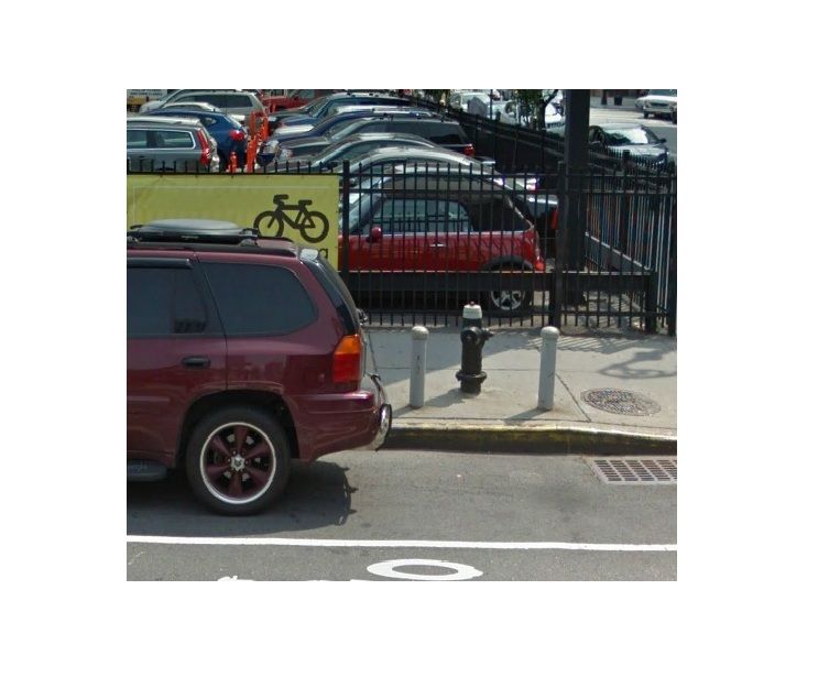
Sensed scene                       Parking map                        Parking
                                                            estimation server                   space map
                                        Private
                                        garage

                                                             Bus
                                                             stop
                             Side
                            street

                                                    Fire                                Illegal parking space
                                                  hydrant                              Legal parking space

                                              Fig. 1: Overview of the proposed system

spaces can be used in the creation of services similar to [5],                  II. ON-STREET PARKING DATA
where these services will on the one hand report availability
                                                                       To demonstrate how on-street parking spaces can be mapped
of legal parking spots and on the other report to parking
                                                                    using parking sensors, we used road side parking data obtained
authorities if illegal parking spots are occupied.
                                                                    from Highland Park, NJ and downtown Brooklyn, NY areas.
In this paper, we address the problem of mapping out street
                                                                    The data from these two data sets is collected using the
parking spaces using car preinstalled parking sensors obtained
                                                                    [5], a system which collects on-street parking availability
by crowdsensing. It is important to stress that this project
                                                                    information. The system in [5] consists of a low cost ultrasonic
differs from the [5] in that the goal of [5] was to collect
                                                                    sensor (Figure 2a), which measures distance from the car to
space occupancy data as opposed to our project where the
                                                                    the nearest obstacle, and the GPS receiver which reports the
main goal is to create legal/illegal parking spot maps, maps
                                                                    location of the sensor measurement. The ultrasonic sensor
which earlier work assumes already exist and are available. A
                                                                    emits ultrasonic waves every 50 ms at the frequency of 43
large number of new generation vehicles possess range finder
                                                                    KHz, providing single range readings from 12 to 255 inches.
parking sensors which help drivers to park their vehicles [9].
                                                                    If an obstacle is detected, the sensor will report the distance
While the vehicle is in motion, these sensors can be used to
                                                                    from the obstacle to the vehicle and in the case that no obstacle
detect the presence or absence of parked vehicles on the street.
                                                                    is detected, the sensor will report a distance of 255 inches.
The sensor measurements can then be reported together with
                                                                    The role of the GPS receiver is to provide time stamps and
the vehicles GPS coordinates (which can be obtained from the
                                                                    location stamps for each sensor measurement. The collected
cars preinstalled GPS device) to the centralized server which
                                                                    sensor measurements and corresponding location stamps form
can estimate if the reported parking spaces are legal or illegal.
                                                                    time series data which represents passes through the streets.
In order to accurately estimate parking maps, the centralized
                                                                    The ultrasonic sensor and GPS receiver were deployed on
server would need several measurements of the same location,
                                                                    several vehicles which were cruising around streets and re-
possibly from several different vehicles. This can be achieved
                                                                    porting parking measurements to the centralized server where
using crowdsensing, an approach that collects large amounts
                                                                    they were preprocessed and used by several algorithms in
of sensing data from crowds. By providing parking sensor
                                                                    order to estimate street parking availability. In addition to
measurements, users can help in mapping the streets into legal
                                                                    the ultrasonic sensor and GPS receiver, a small Sony PS3
and illegal parking spaces similarly to other crowdsensing
                                                                    camera was integrated in order to provide ground truth for
projects where crowdsensing data is used to estimate traffic,
                                                                    parking estimation. The camera was situated just above the
monitor pollution levels in a city, estimate bus arrival times
                                                                    sensor and was aligned together with the sensor (Figure 2a).
and so forth. The diagram of the proposed system is shown
                                                                    It is important to note that the camera was not part of the
in Figure 1.
                                                                    [5] system; it was only used for evaluation and data analysis
The rest of the paper is organized as follows. In section 2,
                                                                    purposes.
we will explain data sets used to demonstrate how parking
maps can be created based on ultrasonic parking sensors and         A. Highland Park data set
give a brief overview of the [5] system which is used to
collect parking data. In section 3 we will present algorithms for      The first parking data set was collected in 2009 in Highland
estimating parking maps from several passes through the same        Park, NJ in three road side parking areas as illustrated in
streets and present results of the evaluation of the algorithms     Figure 3a. Three sensing vehicles collected data during a two
in section 4. Finally in section 5 we discuss in more detail        month period during their daily commutes. They collected
some of the issues we encounter followed by related work in         more than 500 miles of roadside parking data. The data was
section 6 and conclusions in section 7.                             collected only from certain streets in Highland Park (Table
                                                                    I) and this was done by using the concept of trip boxes,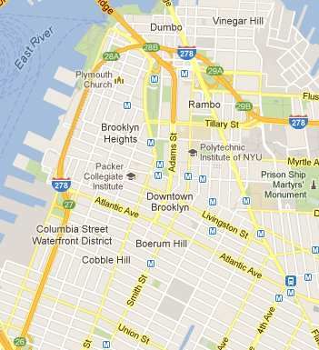
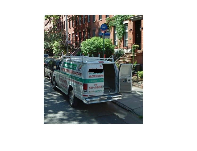
(a) Position of ultrasonic sensor and web camera(b) Vehicle parked on the bus stop on Bergen(c) Vehicle parked to close to fire hydrant on
                                                      Street                                      Schermerhorn Street

                                    Fig. 2: Ultrasonic sensor properties and parking violations
                                                                            TABLE I: Selected streets for both data sets
which represent a rectangular area defined by two latitude and         Street     Street      # of    From       To                           Bicyc
longitude points. As soon as a vehicle enters the area defined          name    length(m)    passes                                           lane
by these points, the sensing vehicle starts collecting data and                            Brooklyn
continues to collect while the vehicle is inside of the box. The      Bergen       608         8     Nevins     Smith                          no
                                                                       Smith       311         8      Dean     Scherm                          yes
trip boxes ensure that data is collected only from streets where       Nevins      382         8     Scherm    Bergen                          no
it is important to estimate parking availability as opposed to         Dean        608         3      Smith    Nevins                          no
areas where parking is available during the whole day. This           Scherm.      608         6      Smith    Nevins                          yes
                                                                      Wychoff      608         3      Smith    Nevins                          no
data set was used in the [5] paper experiments.                        Court       222         6     Atlantic Congress                         no
                                                                                Clinton        394           3         Amity       Living.     no
B. Brooklyn data set                                                                                      High. P.
                                                                                Kilmer         884          10         Plainf.    Truman           no
   The second data set was collected in downtown Brooklyn,                     Raritan         357          20          Third       Fifth          no
NY, and it is used for the first time in this paper. Six sensing               Woodbr.         409          20         Seventh    Eleventh         no
vehicles equipped with the ultrasonic sensor and Sony PS3
webcam were deployed to collect parking data during the                     such as fire hydrants, private garages, side streets, or bus zones.
fall of 2010, over four different work days. The starting                   On the other hand, spaces which are frequently occupied
location for each vehicle was NYU - Poly University, and                    almost every time are likely to be valid parking spaces. Such
each vehicle was assigned a different route to cover an area in             information can be inferred by aggregating available time
downtown Brooklyn but some of the routes had overlapping                    series. In the following sections we will describe our proposed
areas. Figure 3b depicts the location of more than 1.5 million              weighted occupancy rate thresholding algorithm as well as two
points collected during the experiment. Unlike the Highland                 baseline algorithms. Before presenting these algorithms, we
Park data set, in Brooklyn the number of days in which                      will discuss the pre- and postprocessing stages common to all
vehicles were deployed was small but the size of the parking                these algorithms.
area was much larger. As a large, dense city, Brooklyn also
represents a more complex parking landscape than Highland                   A. Baselines, pre- and postprocessing
Park. In this data set, the concept of trip boxes was not                      Since the sensor measurements from different passes are
used. From this large data set, we extracted eight streets in               not necessarily taken at the exact same position, the first step
downtown Brooklyn for which we had at least three passes                    in the preprocessing stage was to spatially discretize streets in
through the same street (Table I). In total, the number of                  one meter cells. Then, all obtained GPS readings and their cor-
data points collected by the [5] in both Highland Park and                  responding sensor measurements are linked with the matching
downtown Brooklyn areas and used in experiments was greater                 space cells. In the case that we have several sensor readings
than 2 million.                                                             associated with one cell (for example a vehicle was standing on
                                                                            the certain spot for several minutes) we take the median value
    III. MAPPING ON-STREET PARKING SPACES
                                                                            of the sensor readings from these locations. However, GPS
              USING AGGREGATION
                                                                            readings are typically accurate up to three meters which can
   Every time a sensing vehicle passes through a street, it can             cause certain sensor readings to be associated with the wrong
collect and report the rangefinder sensor measurement at each               cells. In the next step we discretize sensor measurements. As
location. When several passes through the same street have                  described, the parking sensor provides measurements from 12
been obtained, this will provide us with multiple snapshots of              to 255 inches. Within this range it is possible to detect not
the parking occupancy in this street. To infer from this data               only parked vehicles, but also other objects on the streets
whether a particular road-side spot is a legal parking space, our           such as traffic lights, trees, trash cans, staircases, etc (Figure
algorithm exploits the following key idea: spaces that almost               4a). A common feature for all the objects is that they are
never have parked cars are probably not legal parking spots                 usually positioned behind parked cars. As a first step, we weed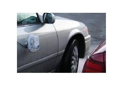
40.525                                                                                     40.705

                                 40.52
                                                                                                                             40.7

                                40.515

                                                                                                                           40.695
                                 40.51

                     Latitude

                                                                                                                Latitude
                                40.505
                                                                                                                            40.69

                                  40.5

                                                                                                                           40.685
                                40.495

                                 40.49                                                                                      40.68
                                   −74.44   −74.435   −74.43    −74.425   −74.42   −74.415   −74.41   −74.405                       −74     −73.995    −73.99     −73.985   −73.98   −73.975
                                                                    Longitude                                                                         Longitude

                                                        (a) Highland Park                                                                 (b) Downtown Brooklyn

                                                               Fig. 3: Locations of the GPS traces for both data sets

out all unnecessary objects by applying a threshold method                                                           location and plot the map of legal/illegal parking spaces.
to time series; everything below the threshold is considered                                                         B. Weighted occupancy rate thresholding approach
as a detected vehicle and it is assigned a value of 0 and
everything above the threshold has a value of 1 and represents                                                          This algorithm is motivated by the observation that not
that nothing was detected on this space in the street. The                                                           all time series from the same street provide equally good
threshold values vary for different streets; for streets without a                                                   information. The time series that have a larger occupancy of
bicycle lane this threshold is set as 100 inches and otherwise                                                       vehicles give us more valuable information as opposed to the
is set to 150 inches. Figure 4b demonstrates histograms of the                                                       time series which were collected while the streets were almost
detected vehicles for streets with and without bicycle lanes                                                         empty. The reasoning behind this is the following: when the
(easily obtained from Google Maps) which we used to select                                                           majority of street parking spaces are occupied, only illegal
appropriate thresholds. Finally after the preprocessing step is                                                      parking spaces tend to remain empty. When many parking
finished we obtain several discretized time series on which we                                                       spots are available it is hard for our algorithm to distinguish
can apply aggregation algorithms.                                                                                    spots that are empty because they are illegal from spots that
As one of the baseline approaches we use the trivial approach                                                        are empty because of a lack of parking demand. The weighted
which estimates that all parking spaces are valid similarly to                                                       occupancy rate thresholding approach utilizes this information
[10]. The trivial approach can be useful to inform us about                                                          to assign more weight to the time series that have high vehicle
the percentage of illegal parking spaces in the street after it is                                                   occupancy than to time series with low vehicle occupancy. An
compared with the ground truth parking maps.                                                                         outline of the proposed algorithm is given in the Algorithm 1.
Another baseline approach which we use to aggregate dis-                                                             The algorithm proceeds as follows: for a given input GPS
cretized time series is occupancy rate thresholding. It decides                                                      and corresponding sensor traces the algorithm first performs
if a certain location is a legal/illegal parking space by taking                                                     preprocessing steps as described before. Then for every time
the average of all time series for that specific location. If                                                        series p we calculate the weight W as the ratio of the
this calculated average is greater than 0.5, then this location                                                      occupied slots to the total slots. In the next step we normalize
is considered as a illegal parking spot and vice versa. The                                                          the weights in order to distinguish between low and high
reasoning behind this approach is that if on average there were                                                      informative time series. Then for every space cell i, the
no parked cars on this location, there is a greater chance that                                                      weighted average of sensor readings S for each time series
this is not a legal parking spot. The reason why the threshold                                                       p was calculated. In order to determine if the parking space
above is set to 0.5 is because even if a lot of places are no                                                        is legal or not we apply the threshold method. Similarly to
parking zones, people tend to temporarily park on fire hydrant                                                       the baseline approach, the resulting aggregated time series is
or bus zones spots as is noticed in the data set.                                                                    smoothed to eliminate small spikes. Finally all spaces are again
At the end of the aggregation phase, the post processing step is                                                     linked to their GPS coordinates and can be plotted in order to
applied to smooth out the resulting time series. The smoothing                                                       obtain a map of legal/illegal parking spots.
method finds all legal parking spaces in the resulting time                                                          It is important to mention that, although this simple algorithm
series that are less than three meters and then converts them                                                        was developed specifically for the purpose of aggregating
to illegal parking spaces. In the same fashion, it converts all                                                      time series for parking map estimation, this algorithm can
illegal spaces to legal if they are less than three meters. The                                                      be generalized to other sensing systems which have multiple
smoothing step is important because it eliminates all parking                                                        sensor readings (time series) from the same locations. For
zones that are too small to be parking spots and vice versa.                                                         example, this approach can be used in aerosol retrieval [11], to
For example, the smallest non-parking zones are several garage                                                       estimate the level of aerosol in the air by combining satellite-
entrances and side streets that are not smaller than 3 meters.                                                       and ground-based sensor measurements.
With the post processing step small spikes that show up in                                                                              IV. EXPERIMENTS
the resulting time series are eliminated and the time series is                                                         The baseline and proposed algorithm are evaluated on both
smoothed. After smoothing we connect each space to its GPS                                                           the Brooklyn and Highland Park data sets. We compared
Row sensor data for part of Bergen Street Histogram for streets with bicycle lane
300 800
Bus zone
600
250
Parked cars 400
200 Fire Hydrant
200
Sesnor range (feet)
Empty space
0
0 50 100 150 200 250 300
150 Sensor range (feet)
Histogram for streets without bicycle lane
2000
100
1500
Traffic light 1000
50
500
0 0
20 40 60 80 100 120 140 0 50 100 150 200 250 300
consecutive sensor measurements
Sensor range (feet)
(a) Raw(before preprocessing) sensor data for the part of Bergen Street (b) Histograms of the detected vehicles for streets with (top) and without bicycle
lanes (bottom)
Fig. 4: Data properties
input : The GPS and sensor traces s 60
Aggregation results for both data sets
output: Array of legal/illegal parking cells 50
Trivial
Baseline
Weighted OCT
1. Discretize GPS traces into N equidistant cells
Classification error (%)
40
2. Assign each sensor value s to the corresponding
30
cell i
3. Apply threshold approach to obtain 0/1 sensor time 20
series 10
4. Calculate weights for each time series p 0
for p ← 1 to P do Dean Wyckoff Bergen Scherm Nevins Clinton Court Smith Kilmer WoodbridgeRaritan
N
P
sp,i Fig. 5: Aggregation results for both data sets
Wp = 1 − i=1 ; labeling straightforward. For fire hydrants, we labeled 5 meters
N (15 feet) on each side of the hydrant as illegal parking spots
end
(according to NYC parking rules). Classification error was
5. Normalize the calculated weights
used as a measure of accuracy where the value of each
for p ← 1 to P do
Wp predicted space cell is compared to the corresponding ground
W̃p = P ; truth space cell. After evaluation we noticed that classification
error is in the range of 5 to 15% depending on the street. The
P
Wp
i=1 error is larger when we have a large number of illegal parking
end spaces such as fire hydrants, garage entrances, or bus zones
6. Apply normalized weights to a each cell that were hard to estimate. Another important factor which
for p ← 1 to N do influenced the classification error is the number of diverse time
P
sˆi =
P
W̃p · sp,i ; series for specific streets; the more time series from different
i=1 periods of the day we have, the easier it was to estimate if
end parking spaces are legal or illegal.
7. Apply threshold to estimate if cell is legal/illegal
parking space Figure 5 shows the results from eight streets in downtown
( Brooklyn. The weighted occupancy rate thresholding approach
1 if (sˆi ≥ threshold
sˆi = out-performs the baseline approaches for the majority of the
0 otherwise streets. Furthermore, for some of the streets (ex. Wyckoff and
8. Smooth out obtained time series. Schermerhorn), baseline approach that averages all time series
Algorithm 1: The weighted occupancy rate threshold-
had very low accuracy (between 30 and 40%) which indicates
ing algorithm
that simple averaging of the time series is not a good approach.
the output of both algorithms to ground truth parking maps. We observed that on several streets both algorithms have the
The ground truth maps are obtained by manually creating same performance such as Dean, Court, and Clinton Streets.
parking maps from satellite images and manually labeling After inspection, we discovered that the time series for all
areas as legal and illegal parking based on satellite and Google passes for those streets were very similar (all taken on the same
Street view imagery. In addition, ground truth maps are also day over a close time period) which caused the weights for the
discretized on the resolution of 1 m similarly to algorithm weighted ORT approach to be very similar. In the case where
output maps. The dimensions of bus stops and entrances all weights are similar, the proposed algorithm behaves the
of parking garages are apparent from these images, making same as the baseline algorithm. When we compare street by
street performance, we notice that the error varies significantly40.6875 40.6905 40.526
Legal parking spaces Legal parking spaces Legal parking spaces
Illegal parking spaces Illegal parking spaces 40.525 Illegal parking spaces
40.687 40.69
40.524
40.6865 40.6895 40.523
40.522
40.686 40.689
Latitude
Latitude
Latitude
40.521
40.6855 40.6885
40.52
40.685 40.688 40.519
40.518
40.6845 40.6875
40.517
40.684 40.687 40.516
−73.991 −73.99 −73.989 −73.988 −73.987 −73.986 −73.985 −73.984 −73.983 −73.9902−73.99−73.9898
−73.9896
−73.9894
−73.9892−73.989
−73.9888
−73.9886
−73.9884 −74.426 −74.424 −74.422 −74.42 −74.418 −74.416 −74.414 −74.412
Longitude Longitude Longitude
(a) Ground truth map for Bergen Street (b) Ground truth map for Smith Street (c) Ground truth map for Kilmer Street
40.688 40.691 40.526
Ground truth (top) Baseline (top) Baseline (top)
Weighted ORT (middle) Weighted ORT (middle) 40.525 Weighted ORT (middle)
40.6875 40.6905
Baseline (bottom) Ground truth (bottom) Ground truth (bottom)
40.524
40.687 40.69
40.523
40.6865 40.6895
40.522
Latitude
Latitude
Latitude
40.686 40.689 40.521
40.52
40.6855 40.6885
40.519
40.685 40.688
40.518
40.6845 40.6875
40.517
40.684 40.687 40.516
−73.991 −73.99 −73.989 −73.988 −73.987 −73.986 −73.985 −73.984 −73.983 −73.9905 −73.99 −73.9895 −73.989 −73.9885 −73.988 −74.426 −74.424 −74.422 −74.42 −74.418 −74.416 −74.414 −74.412
Longitude Longitude Longitude
(d) Estimated map for Bergen Street (e) Estimated Smith Street (f) Estimated map for Kilmer Street
Fig. 6: Ground truth (top) and estimated (bottom) parking maps for three test streets
from street to street for both approaches due to significant approach. From the figure we can observe that the weighted
distinction between the streets. For example, Dean Street is occupancy rate thresholding approach generates more accurate
very narrow and the side where the sensor was measuring had maps than the baseline approach and it is able to accurately
no fire hydrants or bus stops, but only one garage entrance and detect most of the illegal parking spaces.
three intersections. On the other hand, Schermerhorn Street has It will be interesting to see how the proposed algorithm
several fire hydrants, bus stops, and garage entrances. One of compares with other approaches for parking map estimation,
the reasons why the error was slightly larger on Smith Street for example, using GPS traces in cars to see where they stop
is because parking rules were changed in the last couple of for long periods or perhaps participatory sensing where users
years and city authorities installed several new fire hydrants mark spots as legal/illegal as they drive to find an open ”spot”
but left old parking markings visible. This caused many of indicated by the system. However, we were not able to obtain
drivers to park on illegal spots, making those spots hard to data from these approaches in order to perform comparison.
detect. Even during inspection of streets on Google maps we A. Properties of weighted occupancy rate thresholding algo-
noticed quite a few parking violations(Figure 2b and Figure rithm
2c).
Figure 5 also shows results for the Highland Park data set. In the previous section we demonstrate that the proposed
Similarly to the Brooklyn data set, the proposed algorithm per- approach outperformed the trivial and baseline approaches.
forms better than the baseline approach and trivial approach. Now we investigate the behavior of the weighted occupancy
Although we have a larger number of passes in Highland rate thresholding algorithm when we change the number of
Park than in Brooklyn, estimation of the parking maps for time series used for aggregation. In the following experiment
Highland Park was more challenging since Highland Park we used the time series for Bergen Street and we evaluated the
streets are much less occupied and located in a low populated performance of the proposed algorithm for each combination
residential area where a lot of residents park on side streets or of time series. In Figure 7a, we can observe how both the
behind their houses. Thus, most of the time series contained classification error and confidence interval decrease when we
very little information about parked vehicles, which made it add more and more time series. This indicates that the per-
difficult to distinguish between legal and illegal parking spaces formance of weighted occupancy rate thresholding algorithm
after aggregation. Furthermore, Raritan Avenue has a large improves when we receive additional time series.
number of slotted parking spots which were rarely occupied, Next, we investigated how weights of the proposed algorithm
leading to a high percentage of non-parking spaces in that change when we add more data. The weights for each time
street which was hard to estimate. Finally, Figure 6 displays series in each iteration are presented in Figure 7b for one
true and estimated parking maps for baseline and proposed combination of Bergen Street time series. In the first iteration
we have only one time series which has a weight of one. In60 9
mean
0.16
95% confidence interval 8
50
0.19 0.16
7
0.24 0.19 0.17
40
classification error %
6
0.28 0.21 0.17 0.14
5
30 0.40
0.29 0.22 0.18 0.15
4
0.17 0.10 0.07 0.06 0.05 0.04
20 3
0.51 0.41 0.25 0.18 0.14 0.11 0.09
2
10
1 0.49 0.42 0.25 0.18 0.13 0.11 0.09
1
0 0
0 1 2 3 4 5 6 7 8 9 0 1 2 3 4 5 6 7 8 9
# time series
# time series
(a) Performance of weighted occupancy rate thresholding algo- (b) Weights behavior for different number of time series
rithm for different number of time series
Fig. 7: Proposed algorithm properties
the second iteration, we added additional time series which Data sets limitations. Due to the expensive data collection
were similar to the first one and the algorithm estimated process we were able to evaluate the proposed approach only
approximately similar weights of 0.49 and 0.51. As we add on dense urban areas where parking spots are typically full.
more time series the weights are decreasing, giving more In the case of small towns or more suburban areas where
weight to the more informative time series. Finally, after parking occupancy is very low, the proposed algorithm still
all time series were observed the algorithm assigns the final needs to be evaluated. In the case of the Brooklyn data
weight. It is interesting that time series number three received set, the main problem was that the data collection process
the smallest weight in all cases. After inspection, time series lasted only a few days with small time intervals between
number three indicates that on that time of the day there were passes through the same street. This resulted in all time series
only a few parked vehicles on Bergen Street for that specific for a particular street holding very similar information. For
time. If only this time series is available it will be extremely example, for Clinton Street we had three passes of the same
hard to distinguish between illegal parking spaces and legal sensing vehicle in the time period of only a couple of hours.
parking spaces that were not occupied for that time of the The parking situations did not significantly change and the
day. algorithm concluded that all empty spaces at that time were
Finally we examine the fraction of false positive and false illegal. This problem can be solved if more diverse data were
negative for all test streets. The false negative rate in our available, especially in cases where most of the parking spaces
case represents the number of illegal parking spaces that are were occupied (e.g. during night). On the other hand, in the
classified as legal, and vice versa for the false positive ratio. Highland Park data set we had several time series during the
Table II demonstrates these ratios for all test streets. day collected over a larger time period. The main difficulty
TABLE II: False negative and false positive rates in estimating illegal parking spots was the fact that the area
Street name false negative (%) false positive (%) is not as densely populated and parking spaces remain empty
Bergen 3.29 5.76 for most of the day, making estimation more challenging.
Smith 8.36 6.11 Parking maps accuracy. Based on results obtained from
Nevins 3.14 4.19 the evaluation we can pose the question of whether ∼ 90%
Dean 0.66 5.91
Scherm. 9.31 9.31 accuracy is sufficient to use this technique in practice. For
Wychoff 1.32 3.62 applications such as detection of zones with large numbers of
Court 4.50 2.25 illegal spaces for travelers or DOT departments, an accuracy
Clinton 9.14 6.60
Kilmer 0.34 9.39 of ∼90% is more than sufficient. On the other hand, for
Raritan 11.7 3.92 GPS receiver or PARKNET applications which require fine
Woodbr. 5.62 7.82 resolution of parking maps, accuracy of the proposed approach
Average 5.21 5.89
is adequate, especially if we take into account that on average
only ∼5% of the error is due to false negative rate. This
Based on the Table II analysis of false negative rate, we implies that situations where illegal parking space is estimated
notice that only ∼5% of parking spaces will be classified as as legal and which may cause user frustration will be very rare.
legal even though they are illegal. This is very important for Multilane roads. An important issue we encounter is how to
applications that suggest to users where they are allowed to detect legal/illegal parking spaces when sensing vehicles are
park in the streets. passing through multilane streets. Unfortunately, current GPS
V. DISCUSSION receivers are not precise enough to distinguish in which lane
the vehicle is driving. In the data set used in the experiments,
In this section we will discuss in more detail some of the most of the streets are single lane streets and in cases where we
issues we encounter.have multiple lane streets we eliminate the time series in which points of parking sensor readings in our experiments we
the sensing vehicle is changing the lane. In the process of data reached the following conclusions: First, we show how the
analysis, we noticed that if the vehicle is not in the right lane, parking maps can be estimated with an accuracy of ∼90%
sensor measurements are unusually low (the sensing vehicle is from the parking sensor data using proposed weighted oc-
detecting another vehicle that is very close) or unusually high cupancy rate thresholding algorithm. Then, we demonstrated
for longer time periods (the sensing vehicle did not detect that the proposed approach outperforms trivial and baseline
anything because it was far away). Developing an approach approaches on both data sets. Finally, we illustrate how
which will automatically detect these situations remains for accuracy of the proposed algorithms improves by adding more
future work. passes (time series) trough the same street.
Privacy. When we deal with GPS trace data sets, one of
ACKNOWLEDGMENT
the main issues is the question of privacy. Sensing vehicles
must reveal their position to the parking estimation system. The authors would like to thank Patrick Yuen for his help
This can lead to the users home and work locations being re- in data preprocessing and Jelena Coric for her help in editing
vealed simultaneously with their daily patterns. The proposed the paper.
approach [12] addresses the problem of preserving privacy for R EFERENCES
crowdsensing and it can be applied to our problem. In this
[1] Intelligent transportation systems. [Online]. Available: www.its.dot.gov/
paper we do not further address this issue. [2] D. Shoup, “Cruising for parking,” Transport Policy, vol. 13, no. 6, pp.
479–486, 2006.
VI. RELATED WORK [3] ——, “The price of parking on great streets,” University of California
Transportation Center, Tech. Rep., 2011.
In recent years several systems have been developed and [4] Sf-park project. [Online]. Available: http://sfpark.org/
tested for parking space monitoring. Parking garages use [5] S. Mathur, T. Jin, N. Kasturirangan, J. Chandrasekaran, W. Xue,
systems which count the number of vehicles entering/exiting M. Gruteser, and W. Trappe, “Parknet: drive-by sensing of road-side
parking statistics,” in Proceedings of the 8th international conference
the garages and display an estimated number of empty parking on Mobile systems, applications, and services. ACM, 2010, pp. 123–
spaces on the garage entrance message signs [13]. A couple 136.
of interesting approaches were recently proposed, where users [6] Google maps. [Online]. Available: https://maps.google.com/
[7] J. Biagioni and J. Eriksson, “Inferring road maps from gps traces: Survey
can buy and sell privately owned parking spaces [14]. Recently and comparative evaluation,” in Transportation Research Board 91st
two systems which monitor on-street parking spaces were Annual Meeting, no. 12-3438, 2012.
proposed. The first one is SF-park [4], a project in the city of [8] X. Liu, J. Biagioni, J. Eriksson, Y. Wang, G. Forman, and Y. Zhu,
“Mining large-scale, sparse gps traces for map inference: comparison
San Francisco which employs a large number of fixed sensors of approaches,” in Proceedings of the 18th ACM SIGKDD international
for parking space detection and second, the PARKNET project conference on Knowledge discovery and data mining. ACM, 2012, pp.
[5], where low cost ultrasonic sensors coupled with a GPS 669–677.
[9] G. Brosicke, O. Mayer, R. Eri, and H. Seeger, “The automatic parking
receiver were installed in sensing vehicles in order to detect brake.” ATZ Automobiltechnische Zeitschrift, vol. 103, pp. 39–42, 2001.
on-street parked vehicles. It is assumed that parking maps are [10] Primo spot. [Online]. Available: http://www.primospot.com/
already available to the system as noted in the introduction. [11] K. Ristovski, S. Vucetic, and Z. Obradovic, “Uncertainty analysis of
neural-network-based aerosol retrieval,” Geoscience and Remote Sens-
The construction road maps from GPS traces are recognized ing, IEEE Transactions on, vol. 50, no. 2, pp. 409–414, 2012.
as an important problem and in the past couple of years [12] K. Tang, P. Keyani, J. Fogarty, and J. Hong, “Putting people in their
several studies have been done on this topic. Several data place: an anonymous and privacy-sensitive approach to collecting sensed
data in location-based applications,” in Proceedings of the SIGCHI
mining algorithms such as K-means, kernel density estimation conference on Human Factors in computing systems. ACM, 2006,
or trace merging algorithms [7], [15] were proposed in order pp. 93–102.
to estimate road maps from low resolution and low sampling [13] Smart-parking at rockridge bart station. [Online]. Available:
http://www.path.berkeley.edu/ path/research/featured/120804/smart-
traces. As opposed to these approaches, the community in park.html
Open-StreetMaps (OSM) [16] is manually extracting roads [14] Mobileparking. [Online]. Available: https://www.mobileparking.com
from arterial images and GPS traces. However, all proposed [15] L. Cao and J. Krumm, “From gps traces to a routable road map,” in
Proceedings of the 17th ACM SIGSPATIAL International Conference on
approaches focus only on estimating road maps, leaving the Advances in Geographic Information Systems. ACM, 2009, pp. 3–12.
problem of creating parking maps open. [16] Open streetmap. [Online]. Available: http://www.openstreetmap.org
There is a wide variety of applications for traffic state esti- [17] E. Koukoumidis, L. Peh, and M. Martonosi, “Signalguru: leveraging
mobile phones for collaborative traffic signal schedule advisory,” in
mation that use crowdsensing data such as the detection and Proceedings of the 9th international conference on Mobile systems,
prediction of traffic light schedules using smart phone images applications, and services. ACM, 2011, pp. 127–140.
[17], providing real time bus arrival times by distinguishing [18] P. Zhou, Y. Zheng, and M. Li, “How long to wait?: Predicting bus arrival
time with mobile phone based participatory sensing,” in Proceedings of
buses using microphone and GPS sensors [18] or developing the 10th international conference on Mobile systems, applications, and
fuel efficient maps using fuel consumption sensor data [19]. services. ACM, 2012, pp. 379–392.
[19] R. Ganti, N. Pham, H. Ahmadi, S. Nangia, and T. Abdelzaher,
VII. CONCLUSIONS “Greengps: A participatory sensing fuel-efficient maps application,” in
Proceedings of the 8th international conference on Mobile systems,
In this paper we have presented how crowdsensing can be applications, and services. ACM, 2010, pp. 151–164.
used in the mapping of on-street parking spaces to construct
legal/illegal parking maps. Based on the more than 2 millionYou can also read