Computational 4D imaging of light-in-flight with relativistic effects
←
→
Page content transcription
If your browser does not render page correctly, please read the page content below
1072    Vol. 8, No. 7 / July 2020 / Photonics Research                                                          Research Article

Computational 4D imaging of light-in-flight with
relativistic effects
YUE ZHENG,1,2            MING-JIE SUN,1,* ZHI-GUANG WANG,1                     AND    DANIELE FACCIO3
1
  School of Instrumentation Science and Opto-electronic Engineering, Beihang University, Beijing 100191, China
2
  School of Physics, Beihang University, Beijing 100191, China
3
  School of Physics and Astronomy, University of Glasgow, Glasgow G128QQ, UK
*Corresponding author: mingjie.sun@buaa.edu.cn

Received 18 February 2020; revised 31 March 2020; accepted 10 April 2020; posted 10 April 2020 (Doc. ID 390417); published 3 June 2020

      Light-in-flight imaging enables the visualization and characterization of light propagation, which provides
      essential information for the study of the fundamental phenomena of light. A camera images an object by sensing
      the light emitted or reflected from it, and interestingly, when a light pulse itself is to be imaged, the relativistic
      effects, caused by the fact that the distance a pulse travels between consecutive frames is of the same scale as the
      distance that scattered photons travel from the pulse to the camera, must be accounted for to acquire accurate
      space–time information of the light pulse. Here, we propose a computational light-in-flight imaging scheme
      that records the projection of light-in-flight on a transverse x−y plane using a single-photon avalanche diode
      camera, calculates z and t information of light-in-flight via an optical model, and therefore reconstructs its
      accurate (x, y, z, t) four-dimensional information. The proposed scheme compensates the temporal distortion
      in the recorded arrival time to retrieve the accurate time of a light pulse, with respect to its corresponding
      spatial location, without performing any extra measurements. Experimental light-in-flight imaging in a three-
      dimensional space of 375 mm × 75 mm × 50 mm is performed, showing that the position error is 1.75 mm,
      and the time error is 3.84 ps despite the fact that the camera time resolution is 55 ps, demonstrating the feasibility
      of the proposed scheme. This work provides a method to expand the recording and measuring of repeatable
      transient events with extremely weak scattering to four dimensions and can be applied to the observation of
      optical phenomena with ps temporal resolution.
      Published by Chinese Laser Press under the terms of the Creative Commons Attribution 4.0 License. Further distribution of this work
      must maintain attribution to the author(s) and the published article’s title, journal citation, and DOI.
      https://doi.org/10.1364/PRJ.390417

1. INTRODUCTION                                                                   Compared to everyday photography, imaging light-in-flight
Optical imaging of ultra-fast phenomena [1,2] provides critical              is particularly interesting because light is both the medium car-
information for understanding fundamental aspects of the                     rying information to the camera in the form of scattered pho-
world we live in [3–5]. The recording of light-in-flight, which              tons and the object to be imaged itself. In such a scenario, the
enables the visualization and characterization of the propaga-               speed of light cannot be treated as an infinite number, as is
tion of light, is one such example. The capturing of light-                  otherwise true for everyday photography. The recording of such
in-flight, sometimes referred to as transient imaging, was first             events will be significantly observer-dependent and will exhibit
performed with intensity gating [6], and then holographic gat-               spatiotemporal distortions [18–21]. In the context of this work,
ing [7], which selected photons at a specific time by a shutter or           “relativistic effects” refer to such spatiotemporal distortions.
an interference scheme. Outstanding works with various appli-                     To explain this point further, see two examples in Fig. 1. As
cations have been developed based on the time gating principle               shown in Fig. 1(a), two consecutive frames are taken by a cam-
[8–11]. More recently, advances in optical devices have enabled              era, recording a car moving from point A at time 0 to point B
the capture of light-in-flight by recording the arrival of photons           within a time interval Δt. It is worth noting that the actual
in a continuous manner with their corresponding arrival time;                moments when the camera records these two frames are at
such devices include streak cameras [12,13], photonic mixer                  t 1 and Δt  t 2 , and the time interval between these two frames
devices [14,15], and single-photon avalanche diode (SPAD)                    would be Δt  t 2 − t 1 rather than Δt. Nevertheless, because
arrays [16,17].                                                              the speed of light can be treated as infinite compared to the

2327-9125/20/071072-07 Journal © 2020 Chinese Laser Press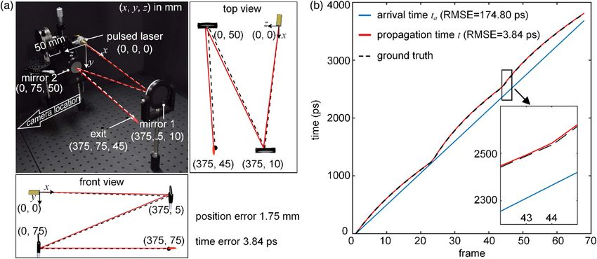
Research Article                                                                        Vol. 8, No. 7 / July 2020 / Photonics Research         1073

                                                                                 point by point three-dimensionally by a distance meter before
                                                                                 performing the actual imaging of light-in-flight [23].
                                                                                     Interestingly, we note that the observer-dependent data of
                                                                                 light-in-flight contains more information than the aforemen-
                                                                                 tioned works have exploited. Here, we demonstrate that the
                                                                                 relativistic effects can be compensated during the imaging of
                                                                                 light-in-flight by further exploiting the (x, y, t a ) data recorded
                                                                                 by a SPAD camera via a strictly built optical model and a com-
Fig. 1. Schematics of difference between imaging (a) a moving car                putation layer to obtain non-distorted time t of a flying light
and (b) a flying light pulse. Δt stands for the time during which the            pulse, without any additional measurements or auxiliary rang-
object moves from position A to position B, and t 1 and t 2 denote the           ing equipment. Simultaneously, the information of an extra
time of flight for the scattered photons to propagate to the camera              dimension, i.e., z dimension, can be retrieved, leading to the
from positions A and B, respectively.                                            observer-independent space-time (x, y, z, t) four-dimensional
                                                                                 (4D) reconstruction of light-in-flight. The proposed scheme
                                                                                 enables the accurate visualization of transient optical phenom-
speed of the car, the camera-measured Δt  t 2 − t 1 can be treated              ena such as light scattering or interaction with materials.
as Δt, which leads to observer-independent results. On the con-
trary, when a light pulse is travelling from A to B, as shown in                 2. EXPERIMENTAL SETUP
Fig. 1(b), the camera-measured time interval Δt  t 2 − t 1 can no               Our experimental system is illustrated in Fig. 2. A 637 nm pulsed
longer be treated as Δt, because t 2 − t 1 is of the same scale as               laser (PicoQuant, LDH-P-635, wavelength 636–638 nm, rep-
Δt. The recorded information of such events is significantly                     etition rate 20 MHz, 1.2 mW, pulse width 68 ps) emits laser
observer-dependent and contains spatiotemporal distortions.                      pulses with 68 ps pulse duration at 20 MHz repetition rate.
     In order to retrieve observer-independent information of                    The pulses propagate across the field of view (FOV) of a
light-in-flight, this relativistic effect (finite light speed of c )             SPAD camera, which consists of a SPAD array (Photon Force
needs to be compensated for to determine the accurate time                       PF32, time resolution 55 ps, pixel resolution 32 × 32, pixel pitch
t when the event actually happens rather than the arrival time                   50 μm, fill factor 1.5%, operating at 5000 frames per second) and
t a at which it is detected by the camera. In holographic light-in-              a camera lens (Thorlabs, MVL4WA, effective focal length
flight imaging, this compensation can be performed using a                       3.5 mm, F/1.4, CS mount). The camera is synchronized to
graphical method based on the ellipsoids of the holodiagram                      the pulsed laser and contains a 32 × 32 array of SPAD detectors,
[22]. A straightforward approach is to simply remove the                         each of which operates in time-correlated single photon counting
time-of-flight, i.e., t 1 and t 2 in Fig. 1, from each measurement               (TCSPC) mode individually, and records the temporal informa-
corresponding to its spatial location, which in turn is measured                 tion of a laser pulse by sensing one of the scattered photons from

Fig. 2. Experimental system for light-in-flight measurement and data processing. (a) In the experiment, the pulsed laser and the SPAD camera are
synchronized via a trigger generator. Placed at z  0 mm, a 636 nm pulsed laser emits pulses across the field of view of the SPAD camera. The SPAD
camera, with a lens of 3.5 mm focal length, is located at z  535 mm. The object focal plane of the camera is the x–y plane at z  0 mm, having a
field of view of 245 mm × 245 mm. The SPAD camera collects the scattered photons from the propagating laser pulses and records a histogram at
each pixel using TCSPC mode. (b) The raw data of the histograms is fitted with a Gaussian distribution. Histograms with widths too large or too
small are discarded (pixels 1 and 2). Malfunctioning pixels with abnormally large counts are also discarded (pixel 4), leaving only effective pixels
(pixel 3). (c) The arrival time of the scattered photons t a in the effective pixels is determined as the peak position of the fitted Gaussian distribution,
and a pixel versus arrival time can be obtained. Consequently, the projection of the light path on the x–y plane, as well as the arrival times along the
path is obtained, forming the (x, y, t a ) three-dimensional data of light-in-flight.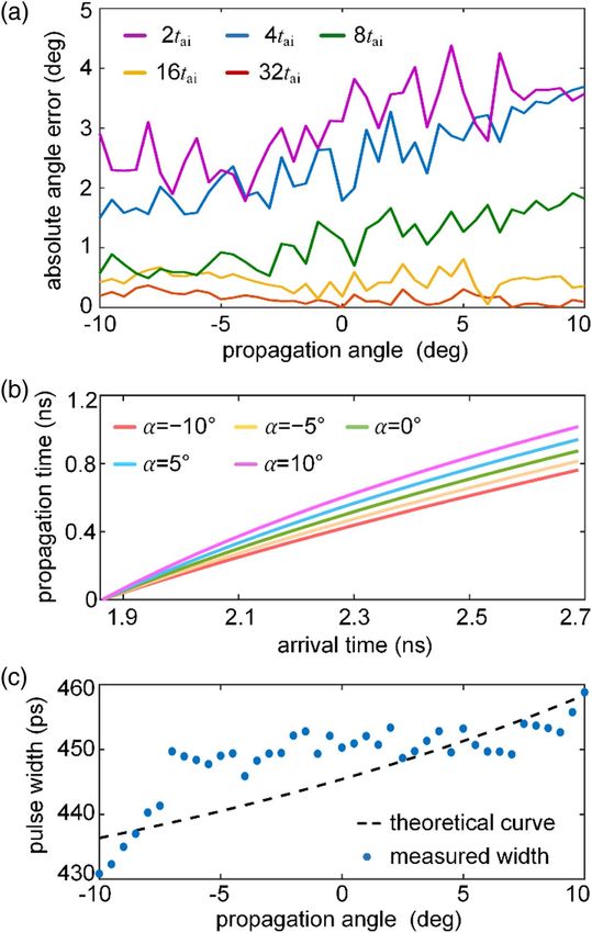
1074     Vol. 8, No. 7 / July 2020 / Photonics Research                                                                Research Article

the laser pulse. By accumulating data over multiple detection
frames, each pixel obtains a temporal histogram of scattered pho-
tons whose total number represents the scattering intensity of the
laser pulse at the corresponding spatial location, and the histo-
gram shape indicates the arrival time of the scattered photons.
Combining the histogram data recorded by the pixels of the
SPAD camera, the projection of the light-in-flight on the x–y
plane inside the FOV of SPAD camera can be reconstructed [24].
    The accurate estimation for the arrival time t a of the scat-
tered photons at each pixel of the SPAD camera is important           Fig. 3. Optical model for the computation of propagation time t. α
for the light-in-flight reconstruction. Gaussian fitting is per-      and θ are the angles of ∠CBG and ∠BAF , respectively. s and l are the
formed on the raw histogram data at each pixel to suppress            lengths of BA and BE, respectively. BE is the projection of BD on the
the statistical random noise of photon counting. Under the            reference plane (RP).
assumption that the background light and dark count of the
SPAD camera, whose temporal distribution is quasi-flat, add
a bias to the histogram, a constant term is added to the                                   qffiffiffiffiffiffiffiffiffiffiffiffiffiffiffiffiffiffiffiffiffiffiffiffiffiffiffiffiffiffiffiffiffiffiffiffiffiffiffiffiffiffiffiffiffiffiffiffiffiffiffiffiffiffiffiffi
Gaussian polynomial during the fitting in order to improve                      ta  t     s2 ∕c 2  t 2 − 2st sinα  θ∕c ,                         (1)
the estimation accuracy of the arrival time. During the data
                                                                      where s is the distance from B to the camera A and can be cal-
processing, if the width of a fitted Gaussian curve is much larger
                                                                      culated using the recorded arrival time of the pixel correspond-
or smaller than the expected width, the corresponding pixel is
                                                                      ing to B. θ is the angle between AB and AF, and can be
assumed to be malfunctioning or extremely noisy, and is there-
                                                                      calculated using the value of s and the known camera FOV.
fore discarded. Furthermore, the systematic overall delay, which
                                                                      The second term of Eq. (1) represents the time interval that
is mainly caused by electronic jitter of the related devices and is
                                                                      light propagates from D to A, in which the propagation angle
different for each pixel, is compensated by a temporal offset for
                                                                      α is defined as the angle between the light path BD and its
each effective Gaussian curve. The offset for the corresponding
pixel is determined as the temporal difference between the mea-       projection BE on reference plane. t and α are related via the
sured peak position of the corresponding pixel and its theoreti-      following equation:
cal value, which is measured when the camera is uniformly                                  1          s · l · cos θ
                                                                                      t                                ,                              (2)
illuminated with a collimated and expanded pulsed laser.                                   c l · sin α  s · cosα  θ
    Once the raw histogram data is Gaussian fitted and the
                                                                      where l is the length of BE and can be calculated using the value
temporal-delay is compensated at each pixel, the peak of its
                                                                      of s and the known camera FOV. By substituting Eq. (2) into
histogram is determined, which represents the arrival time t a of
                                                                      Eq. (1), the arrival time t a and the propagation angle α form a
the light recorded at the corresponding pixel. As shown in
                                                                      one-to-one relationship. BG is the projection of BC on RP, and
Fig. 2, the path of a laser pulse propagating through the FOV
                                                                      can be recorded by the SPAD camera, forming 32 photon-
of the camera is reconstructed as its projection on the x–y plane,
and the arrival time t a along that path is estimated, forming the    counting histograms. The arrival time t ai of the ith histogram
(x, y, t a ) three-dimensional (3D) data of light-in-flight.          can be used to yield a propagation angle αi . However, due to
                                                                      noise contained in the recorded data, 32 t ai yields 32 different
                                                                      αi , which should be identical theoretically. The optimal estima-
3. OPTICAL MODEL AND COMPUTATIONAL                                    tion of the propagation angle α is then calculated as the value
LAYER                                                                 having the minimum root-mean-square error (RMSE), with 32
In order to transfer the arrival time t a distorted by the relativ-   resulting αi .
istic effects to the accurate time t at which the light pulse              Using the calculated propagation angle α, the propagation
actually is at a given position, an optical model is built as shown   time t can be determined for each recorded (x, y). Furthermore,
in Fig. 3. For simplicity, the computation is based on the            the z information of the corresponding (x, y) can also be
assumption that light propagates in air, though it works for          retrieved via the knowledge of α. Therefore, the observer-
any uniform and homogenous medium in which the light                  independent 4D (x, y, z, t) information of light-in-flight is
propagates in a straight line at a fixed velocity. The moment         reconstructed.
at which a light pulse enters the FOV of the camera is defined             The procedure to reconstruct multiple light paths is illus-
as t 0  0 s, which makes t the propagation time from the en-         trated in Fig. 4. The light path from the laser emitting point
tering position to where it is now. t will be referred as propa-      to Mirror 1 is denoted as LP1, and the consecutive paths from
gation time hereafter. The x–y plane containing the entering          Mirror 1 to Mirror 2 and from Mirror 2 to the exit are denoted
point is defined as the reference plane. If a light pulse propa-      as LP2 and LP3, respectively. The light paths can be recon-
gates from B towards C, and its arrival time at an arbitrary point    structed one after another sequentially with their corresponding
D is recorded, this arrival time t a will correspond to a timespan    propagation angles and reference planes. As shown in Fig. 4(a),
of light traveling from B to D and then scattering to A (while        the x–y plane at z  0, containing the laser emitting point, is
the propagation time t of the light pulse corresponds to the          defined as the reference plane 1 (RP1). The projection of LP1
time during which light travels from B to D). These times,            in RP1, denoted as PP1, with its spatiotemporal information, is
t a and t, satisfy the equation                                       recorded by the SPAD camera. Using the propagation angle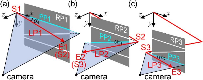
Research Article                                                               Vol. 8, No. 7 / July 2020 / Photonics Research      1075

Fig. 4. Reconstruction procedure for consecutive light paths.
(a) For light path 1 (LP1), the reference plane (RP1) is the x–y plane
containing the starting point 1 (S1). The spatial location of the pro-
jection (PP1), propagation angle, and ending point (E1) of LP1 are
determined using the proposed geometric model. (b) E1 is used as
S2 for the reconstruction of LP2, and RP2 is the x–y plane containing
S2. The equation of LP2 and the position of E2 can be obtained. (c) In
the same manner, LP3 and E3 are determined with RP3.

estimation procedure just described, α1 can be estimated, and
the observer-independent 4D (x, y, z, t) information of LP1 is
reconstructed with the starting point of LP1 (S1) and ending
point of LP1 (E1) determined. As shown in Fig. 4(b), the start-
ing point S2 of LP2 is determined as E1 and the reference plane
2 (RP2) is defined as the x–y plane containing E1. In the same
manner, α2 and the observer-independent 4D information of
LP2 are calculated. Using the ending point E2 of LP2 as the
starting point of LP3 (S3), the reference plane 3 (RP3) of LP3
is defined as shown in Fig. 4(c). Similarly, α3 and the 4D
                                                                         Fig. 5. Experimental results of the propagation angle estimation.
information of LP3 can be retrieved. The full evolution of
                                                                         (a) Angle error resulting from using different numbers of t ai for
light-in-flight in the FOV of the camera is then reconstructed           the estimation of α. (b) Calculated propagation time t with respect
in (x, y, z, t).                                                         to arrival time t a at different propagation angles. (c) The variation
                                                                         of measured full width at half maximum for a laser pulse with respect
4. RESULTS                                                               to its propagation angle α, caused by the relativistic effects.
A. Propagation Angle Estimation
An experiment is performed using the setup in Fig. 2 to evalu-
ate the estimation accuracy of α before performing the 4D                the ground truth when different numbers of t ai are used in the
light-in-flight reconstruction. In this experiment, laser pulses         estimation. As one would expect, 2 t ai yield the largest mean
propagate horizontally, i.e., parallel to the x direction, through       error, which is 3.03°, and 32 t ai give the smallest, which
the center of the camera FOV with a propagation angle α                  is 0.15°.
gradually adjusted from −10° to 10° with a 0.5° step (positive               Figure 5(b) shows the relationship between the measured
is towards the camera and negative is away from the camera).             arrival time t a and the actual propagation time t under the
For each angle, measurements are acquired for 200 s with an              influence of different propagation angles. Figure 5(c) demon-
exposure time of 200 μs for each detection frame. The averaged           strates how relativistic effects distort the measured pulse width
photon count of the SPAD camera is 10−5 photon per pulse per             of a laser pulse. The variation of the pulse width is indistin-
pixel, which satisfies the photon-starved condition required for         guishable when the propagation angle is between −6° and 6°
TCSPC mode. A total of 20 measurements are performed, and                due to the temporal discretization of the SPAD camera, whose
the resulting α is the averaged value of these 20 measurements.          time bin is 55 ps. Nevertheless, the experimental results are in
    During the experiment, the x–y plane containing the                  good agreement with the theoretical curve. Furthermore, the
laser-emitting point is selected to be the reference plane. The          results yield a measured full width at half maximum (FWHM)
histogram of any malfunctioning pixels is discarded and its              pulse width of 65 ps after deconvolving the systematic impulse
corresponding arrival time t a is determined as the linear inter-        respond function from the Gaussian fitted recording data,
polated value of the arrival times from the neighboring pixels. It       which is close to the 68 ps pulse width given by the laser
is worth mentioning that theoretically the propagation angle α           manual.
can be estimated using one or several arrival times t a [25,26].
However, due to the discrete nature of the temporal measuring            B. Light-in-Flight Reconstruction
with the SPAD camera and the noise recorded during a prac-               A second experiment is then performed to reconstruct light-in-
tical experiment, the greater number of t ai are involved in the         flight in a 3D space of 375 mm × 75 mm × 50 mm, where the
calculation, the more accurate the estimated α will be. Figure 5(a)      pulses are emitted from a laser and reflected by two mirrors to
shows the angular errors of the estimated propagation angle α to         generate three consecutive light paths across the FOV of the
1076 Vol. 8, No. 7 / July 2020 / Photonics Research Research Article
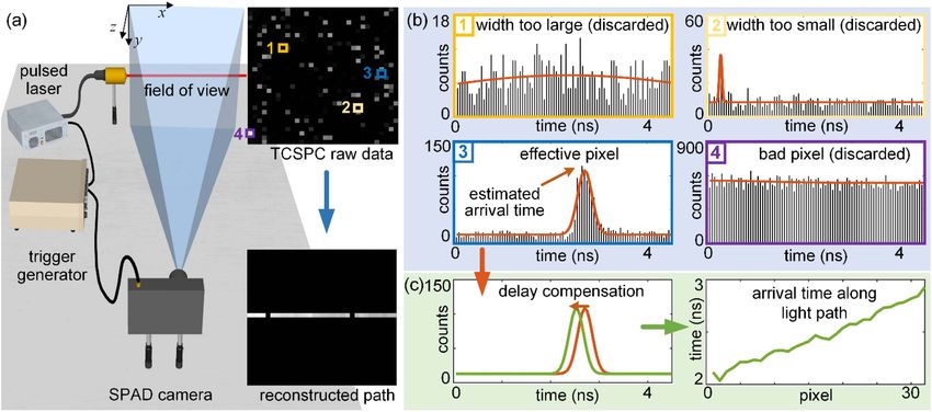
Fig. 6. Experimental 4D reconstruction of light-in-flight. (a) A reconstruction of a laser pulse reflected by two mirrors is demonstrated.
The RMSEs of the reconstruction (red line) to the ground truth (dashed line) in position and time are 1.75 mm and 3.84 ps, respectively.
(b) The difference between the calculated propagation time t (red line) and measured arrival time t a (blue line) at each recorded frame. The
propagation time is in good agreement with the ground truth (dashed line), demonstrating a feasible compensation for the relativistic effects
via the proposed scheme.
SPAD camera. In the experiment, there is a 40 mm distance Figure 6(b) shows the difference between the calculated
between the FOV and any optical elements (e.g., the laser propagation time t (red line) and the measured arrival time
source and the mirrors) in order to avoid spurious scattering t a (blue line) at each recorded frame (55 ps time interval) of
of light into the measurement. The emitting point of the pulsed the SPAD camera, where the arrival time t a has been biased
laser is selected as (0,0,0) of the x–y–z coordinate for calcula- so that it starts at 0 ps at the first frame. The measured arrival
tion. The object focal plane of the SPAD camera is determined time t a has been successfully compensated to be the observer-
to be the x–y plane at z 0. Using the same configuration independent propagation time t, which is in a good agreement
as before, the SPAD camera records the observer-dependent with the ground truth (dashed line). The temporal RMSE to
(x, y, t a ) information of the three light paths inside the FOV. the ground truth is significantly improved from 174.80 to
The reconstruction of light-in-flight is performed by sequen- 3.84 ps.
tially determining the light paths from laser emitting point to
Mirror 1, to Mirror 2, and then to the exiting point. The
reconstruction procedure is given in previous section. 5. DISCUSSION AND CONCLUSION
Figure 6(a) shows the reconstructed propagation of the laser The estimation of propagation angle is crucial to the light-in-
pulse in the x–y–z space, which is overlaid onto a photograph flight reconstruction in this work, and we have demonstrated
of the experimental setup. The instantaneous positions (x, y, z) accurate estimations of propagation angle from −10° to 10°.
of the laser pulse in path are reconstructed with an accuracy of Theoretically, the proposed approach can be used to estimate
1.75 mm RMSE with respect to the ground truth in a 3D space any angle between 90°, not including 90°. Practically, there
of 375 mm × 75 mm × 50 mm. The propagation times t of are two major aspects, noise and diffusion, to consider when
the light pulse are estimated with an accuracy of 3.84 ps, which measuring a steep angle. On the noise aspect, the reconstruc-
is determined as the difference between the ground truth and tion will be even more accurate with a steeper angle because the
the estimated propagation times t, calculated using Eq. (2). relativistic effect is more obvious and the difference between the
The 3.84 ps accuracy is dramatically smaller compared to measured data of two adjacent pixels is easier to be recorded
the 55 ps time resolution of the SPAD camera. The reason above the noise. An accurate reconstruction at a smaller angle
for this improvement lies in the fact that the inaccuracy caused is more difficult to achieve because the milder distortion can be
by the discrete temporal measurements and the experimental easily drowned in the systematic noise. From the diffusion as-
noise is suppressed during the estimation of each propagation pect, a forward steep angle increases the signal-to-noise ratio of
angle α, which involves 32 measured arrival times t a rather than the measured data while a backward steep angle decreases it.
one. The full evolution of the laser pulse propagation can be The proposed method has the assumption that the light-
found in Visualization 1. The FWHM of the propagating laser in-flight to be reconstructed happens in a uniform and homog-
pulse, which is the deconvolved result of the systematic impulse enous medium, where light propagates in a straight line at a
respond function from the Gaussian fitted recording data, is fixed velocity. However, it is also possible to reconstruct self-
approximately 70 ps, consistent with the specification of bending light beams, such as Airy beams [27], in a differential
the laser. manner. That is, the self-bending light path of the Airy beam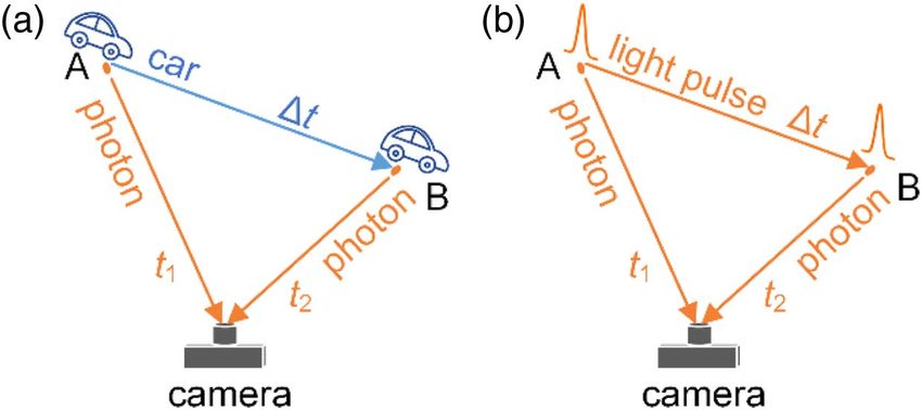
Research Article                                                               Vol. 8, No. 7 / July 2020 / Photonics Research           1077

propagation viewed as a combination of many tiny straight              low scattering from 3D to 4D. It can also be applied to observe
paths, each of which can then be reconstructed individually            optical phenomena which pose a difficulty for other imaging
by the proposed method.                                                schemes, e.g., the behavior of light in micro- or nanostructures
    The position error for a reconstructed light path is mainly        and the interaction between light and matter.
determined by the estimation accuracy of the propagation angle
and the recorded light path projection on a SPAD camera.               Funding. National Natural Science Foundation of China
The estimation accuracy of the propagation angle can be fur-           (61922011, 61675016); Engineering and Physical Sciences
ther improved by taking more measurements or by using a                Research Council (EP/M01326X/1).
camera with lower noise. The accuracy of the recorded light
path projection is limited by the pixel resolution (32 × 32)           Disclosures. The authors declare no conflicts of interest.
and fill factor (1.5%) of the SPAD camera. In particular, when
a light pulse is propagating in a quasi-horizontal x direction,
the small variation in the y direction cannot be spatially re-         REFERENCES
solved by the SPAD camera, which accumulates as the light               1. L. Gao, J. Liang, C. Li, and L. V. Wang, “Single-shot compressed ultra-
pulse propagates and degrades the resulting accuracy of the                fast photography at one hundred billion frames per second,” Nature
reconstruction. A newly developed SPAD camera with a                       516, 74–77 (2014).
256 × 256 pixel resolution and 61% fill factor [28] will improve        2. T. Gorkhover, S. Schorb, R. Coffee, M. Adolph, L. Foucar, D. Rupp, A.
                                                                           Aquila, J. D. Bozek, S. W. Epp, B. Erk, L. Gumprecht, L. Holmegaard,
the reconstruction accuracy of the proposed light-in-flight                A. Hartmann, R. Hartmann, G. Hauser, P. Holl, A. Hömke, P.
imaging system. A backside-illuminated multi-collection-gate               Johnsson, N. Kimmel, K.-U. Kühnel, M. Messerschmidt, C. Reich,
silicon sensor can also be used in light-in-flight imaging [29]            A. Rouzée, B. Rudek, C. Schmidt, J. Schulz, H. Soltau, S. Stern,
to provide a higher fill factor, larger photoreceptive area, and           G. Weidenspointner, B. White, J. Küpper, L. Strüder, I. Schlichting,
higher spatial resolution, with a temporal resolution currently            J. Ullrich, D. Rolles, A. Rudenko, T. Möller, and C. Bostedt,
                                                                           “Femtosecond and nanometre visualization of structural dynamics
of 10 ns, but its sensitivity is not as good as a SPAD camera.             in superheated nanoparticles,” Nat. Photonics 10, 93–97 (2016).
However, the ultimate limit for temporal resolution of these            3. M. B. Bouchard, B. R. Chen, S. A. Burgess, and E. M. C. Hillman,
cameras implies that in the future, sub-ns temporal resolution             “Ultra-fast multispectral optical imaging of cortical oxygenation, blood
could be achievable, thus allowing precise light-in-flight mea-            flow, and intracellular calcium dynamics,” Opt. Express 17, 15670–
                                                                           15678 (2009).
surements with just one single laser shot, as shown in the
                                                                        4. C.-M. Liu, T. Wong, E. Wu, R. Luo, S.-M. Yiu, Y. Li, B. Wang, C. Yu, X.
proof-of-concept work by Etoh et al. [29].                                 Chu, K. Zhao, R. Li, and T.-W. Lam, “SOAP3: ultra-fast GPU-based
    In summary, we have proposed a computational imaging                   parallel alignment tool for short reads,” Bioinformatics 28, 878–879
scheme to achieve the reconstruction of light-in-flight in                 (2012).
observer-independent 4D (x, y, z, t) by recording the scattered         5. J. Liang and L. V. Wang, “Single-shot ultrafast optical imaging,” Optica
                                                                           5, 1113–1127 (2018).
photons of the light propagation with a SPAD camera and                 6. J. A. Giordmaine, P. M. Rentzepis, S. L. Shapiro, and K. W. Wecht,
compensating the relativistic effects via an optical model-based           “Two-photon excitation of fluorescence by picosecond light pulses,”
computation layer. The relativistic effects in this context refer to       Appl. Phys. Lett. 11, 216–218 (1967).
the spatiotemporal distortion caused by the fact that the speed         7. N. Abramson, “Light-in-flight recording by holography,” Opt. Lett. 3,
                                                                           121–123 (1978).
of light needs to be treated as a finite number in certain sce-         8. T. L. Cocker, D. Peller, P. Yu, J. Repp, and R. Huber, “Tracking the
narios such as transient imaging. The estimation of the light              ultrafast motion of a single molecule by femtosecond orbital imaging,”
propagation angle α, which is crucial to the 4D light-in-flight            Nature 539, 263–267 (2016).
reconstruction, has a mean error of 0.15° for the range from            9. K. Goda, K. K. Tsia, and B. Jalali, “Serial time-encoded amplified
                                                                           imaging for real-time observation of fast dynamic phenomena,”
−10° to 10°. In the reconstruction of the light-in-flight in a             Nature 458, 1145–1149 (2009).
3D space of 375 mm × 75 mm × 50 mm, the temporal accu-                 10. K. Nakagawa, A. Iwasaki, Y. Oishi, R. Horisaki, A. Tsukamoto, A.
racy is improved from 174.80 ps of the distorted arrival time to           Nakamura, K. Hirosawa, H. Liao, T. Ushida, K. Goda, F. Kannari,
                                                                           and I. Sakuma, “Sequentially timed all-optical mapping photography
3.84 ps of the compensated propagation time. The spatial
                                                                           (STAMP),” Nat. Photonics 8, 695–700 (2014).
accuracy of the reconstruction is 1.75 mm, which is better             11. T. Kakue, K. Tosa, J. Yuasa, T. Tahara, Y. Awatsuji, K. Nishio, S. Ura,
than both the 8 mm transverse spatial resolution determined                and T. Kubota, “Digital light-in-flight recording by holography by use of
by the optical setup of the system and the 16.5 mm longitude               a femtosecond pulsed laser,” IEEE J. Sel. Top. Quantum Electron. 18,
                                                                           479–485 (2012).
spatial resolution determined by the 55 ps time resolution of
                                                                       12. A. Velten, D. Wu, A. Jarabo, B. Masia, C. Barsi, C. Joshi, E. Lawson,
the SPAD camera. The improvement is mainly achieved by                     M. Bawendi, D. Gutierrez, and R. Raskar, “Femto-photography: cap-
the accurate estimation of the propagation angle α, where the              turing and visualizing the propagation of light,” ACM Trans. Graph. 32,
random-natured noise and the inaccuracy of discrete measure-               44 (2013).
                                                                       13. L. Zhu, Y. Chen, J. Liang, Q. Xu, L. Gao, C. Ma, and L. V. Wang,
ment are suppressed by estimation involving multiple measure-
                                                                           “Space- and intensity-constrained reconstruction for compressed
ments. The accurately estimated propagation angle can be                   ultrafast photography,” Optica 3, 694–697 (2016).
further exploited to correct other distorted measurements.             14. F. Heide, M. B. Hullin, J. Gregson, and W. Heidrich, “Low-budget tran-
    The proposed 4D imaging scheme is applicable to the                    sient imaging using photonic mixer devices,” ACM Trans. Graph. 32,
reconstruction of light-in-flight for other circumstances, such            45 (2013).
                                                                       15. A. Kadambi, R. Whyte, A. Bhandari, L. Streeter, C. Barsi, A.
as light traveling inside a cavity or interacting with other ma-           Dorrington, and R. Raskar, “Coded time of flight cameras: sparse
terials. This work provides the ability to expand the recording            deconvolution to address multipath interference and recover time
and measuring of repeatable ultra-fast events with extremely               profiles,” ACM Trans. Graph. 32, 167 (2013).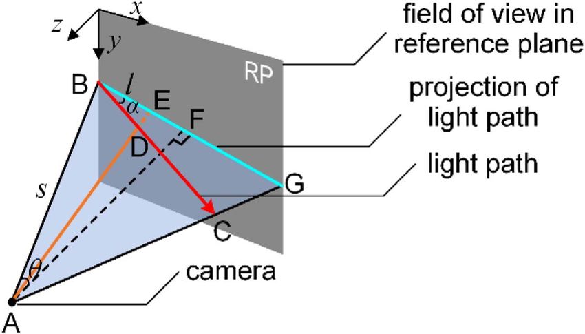
1078      Vol. 8, No. 7 / July 2020 / Photonics Research                                                                    Research Article

16. C. Niclass, M. Gersbach, R. Henderson, L. Grant, and E. Charbon, “A          23. A. Jarabo, B. Masia, A. Velten, C. Barsi, R. Raskar, and D. Gutierrez,
    single photon avalanche diode implemented in 130-nm CMOS tech-                   “Relativistic effects for time-resolved light transport,” Comput. Graph.
    nology,” IEEE J. Sel. Top. Quantum Electron. 13, 863–869 (2007).                 Forum. 34, 1–12 (2015).
17. D. Bronzi, F. Villa, S. Tisa, A. Tosi, F. Zappa, D. Durini, S. Weyers, and   24. G. Gariepy, N. Krstajić, R. Henderson, C. Li, R. R. Thomson, G. S.
    W. Brockherde, “100000 frames/s 64 × 32 single-photon detector                   Buller, B. Heshmat, R. Raskar, J. Leach, and D. Faccio, “Single-
    array for 2-D imaging and 3-D ranging,” IEEE J. Sel. Top. Quantum                photon sensitive light-in-fight imaging,” Nat. Commun. 6, 6021 (2015).
    Electron. 20, 354–363 (2014).                                                25. M. Laurenzis, J. Klein, and E. Bacher, “Relativistic effects in imaging
18. J. M. Hill and B. J. Cox, “Einstein’s special relativity beyond the speed        of light in flight with arbitrary paths,” Opt. Lett. 41, 2001–2004 (2016).
    of light,” Proc. R. Soc. A 468, 4174–4192 (2012).                            26. M. Laurenzis, J. Klein, E. Bacher, N. Metzger, and F. Christnacher,
19. A. Velten, D. Wu, A. Jarabo, B. Masia, C. Barsi, E. Lawson, C. Joshi,            “Sensing and reconstruction of arbitrary light-in-flight paths by a rela-
    D. Gutierrez, M. G. Bawendi, and R. Raskar, “Relativistic ultrafast ren-         tivistic imaging approach,” Proc. SPIE 9988, 998804 (2016).
    dering using time-of-flight imaging,” in ACM SIGGRAPH 2012 (2012),           27. G. A. Siviloglou, J. Broky, A. Dogariu, and D. N. Christodoulides,
    paper 41.                                                                        “Observation of accelerating Airy beams,” Phys. Rev. Lett. 99,
20. M. Laurenzis, J. Klein, E. Bacher, and N. Metzger, “Multiple-return              213901 (2007).
    single-photon counting of light in flight and sensing of non-line-of-sight   28. I. Gyongy, N. Calder, A. Davies, N. A. W. Dutton, R. R. Duncan, C.
    objects at shortwave infrared wavelengths,” Opt. Lett. 40, 4815–4818             Rickman, P. Dalgarno, and R. K. Henderson, “A 256 × 256, 100-kfps,
    (2015).                                                                          61% fill-factor SPAD image sensor for time-resolved microscopy
21. M. Clerici, G. C. Spalding, R. Warburton, A. Lyons, C. Aniculaesei,              applications,” IEEE Trans. Electron. Devices 65, 547–554 (2018).
    J. M. Richards, J. Leach, R. Henderson, and D. Faccio, “Observation          29. T. G. Etoh, T. Okinaka, Y. Takano, K. Takehara, H. Nakano, K.
    of image pair creation and annihilation from superluminal scattering             Shimonomura, T. Ando, N. Ngo, Y. Kamakura, V. T. S. Dao, A. Q.
    sources,” Sci. Adv. 2, e1501691 (2016).                                          Nguyen, E. Charbon, C. Zhang, P. De Moor, P. Goetschalckx, and
22. N. Abramson, “Light-in-flight recording 3: compensation for optical              L. Haspeslagh, “Light-in-flight imaging by a silicon image sensor:
    relativistic effects,” Appl. Opt. 23, 4007–4014 (1984).                          toward the theoretical highest frame rate,” Sensors 19, 2247 (2019).
You can also read