End-to-end measurements over GPRS-EDGE networks
←
→
Page content transcription
If your browser does not render page correctly, please read the page content below
End-to-end measurements over GPRS-EDGE networks
Juan Andrés Negreira Javier Pereira Santiago Pérez
Facultad de Ingenierı́a, Facultad de Ingenierı́a, Facultad de Ingenierı́a,
Universidad de la República Universidad de la República Universidad de la República
Montevideo, Uruguay Montevideo, Uruguay Montevideo, Uruguay
javierp@fing.edu.uy
Pablo Belzarena
Facultad de Ingenierı́a,
Universidad de la República
Montevideo, Uruguay
belza@fing.edu.uy
ABSTRACT 1. INTRODUCTION
In the last years, QoS (Quality of Service) parameter es- Today cellular services include voice communications, email,
timation has become a main research area in networking sms, audio and video streaming and mobile TV. This situ-
due to a continuous growth of the Internet. End-to-end ation has been generated by the increase in cellular access
active measurement is one of the topics that focuses on bandwidth. This type of services have strong constraints
this research area. However, these measurement method- in performance and quality. To deal with this constraints a
ologies have focused on end-to-end measurements over the model that analyzes the end-to-end performance of a GPRS-
wired Internet. The development of cellular data services EDGE connection is necessary. Unfortunately, the analyti-
is shifting the resarch focus on QoS from wired to wireless cal models that have been developed to analyze the perfor-
networks. End-to-end measurement methodologies of cellu- mance of cellular systems make strong simplifications. They
lar networks have some issues that are not considered by can only be used to get a rough dimension of the system, but
traditional measurement techniques. This paper analyzes not to analyze the end-to-end performance of a particular
these issues and suggests an end-to-end active measurement data flow.
methodology that deals with these particular problems. The End-to-end measurements of wired IP networks has been
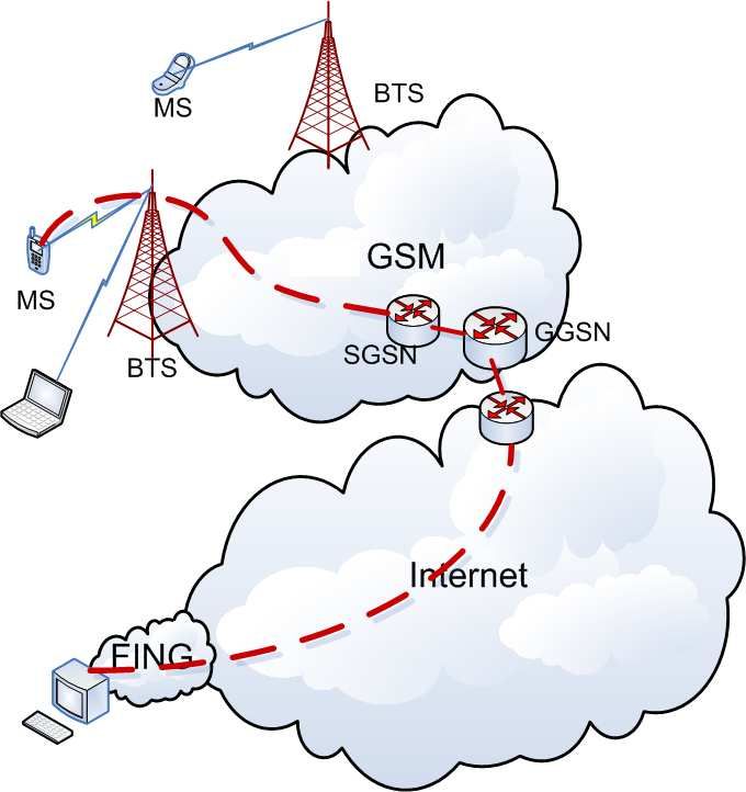
proposed research and measurement methodology is based an important area of research during last years. Therefore,
on a GSM (Global System for Mobile Communications) until last years, the focus was only on wired networks and
network, particularly on data services on a GPRS-EDGE not on wireless networks.
(General Packet Radio Service/Enhanced Data Rates for End-to-end measurements of GPRS-EDGE networks have
GSM Evolution) network. Several experiments in different some particular problems that are not considered in the
situations have been done in a real cellular network. These wired case. For example, the spectrum resource sharing
experiments have tested the performance of the methodol- adds some special issues, as well as the priority of the voice
ogy in different data access conditions. traffic.
The focus of this work is on end-to-end GPRS-EDGE
networks capacity estimation and some other important per-
Categories and Subject Descriptors formance issues. This work suggests a methodology for end-
C.4 [Performance of Systems]: Measurement techniques, to-end measurements of this kind of networks. Based on
Performance attributes. this methodology a software tool was developed. Using that
tool some experiments have been done to estimate different
performance metrics in a GPRS-EDGE network.
General Terms The paper is organized as follows. A summary about the
Network performance, Algorithms. state of art concerning end-to-end measurements over IP
networks is in Section 2. An explanation of important pa-
rameters to measure over GPRS-EDGE is done in Section
Keywords 3. The measurements issues over GPRS-EDGE networks
Performance, QoS, GSM, GPRS-EDGE. are presented in Section 4. An algorithm which deals with
the matters presented in Section 4 is explained in Section 5.
The implemented measurement system is explained in Sec-
tion 6. Some results obtained with this system are presented
Permission to make digital or hard copies of all or part of this work for in Section 7. In Section 8, the influence of the transport
personal or classroom use is granted without fee provided that copies are layer protocols on the throughput measurement is studied.
not made or distributed for profit or commercial advantage and that copies
Finally, the paper is concluded in Sections 9 and 10.
bear this notice and the full citation on the first page. To copy otherwise, to
republish, to post on servers or to redistribute to lists, requires prior specific
permission and/or a fee. 2. RELATED WORKS
LANC ’07 October 10-11, San Jose, Costa Rica
Copyright 2007 ACM 978-1-59593-907-4/07/0010 ...$5.00. The main research topics on end-to-end measurements on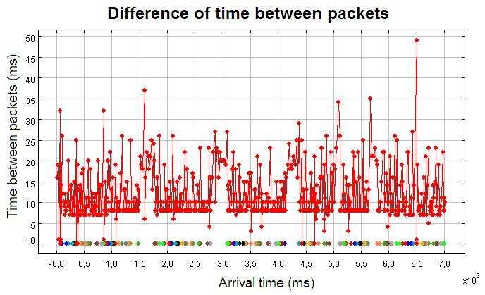
the Internet are:                                                     • Round Trip Time (RTT)
                                                                      • Jitter
Link capacity or bottleneck link capacity estimation in
a network path.                                                      These parameters will be estimated by sending probe packet
   There are many suggested procedures in order to estimate        pairs of constant size $ at constant rate. The inter-arrival
the capacity of a wired link. Main techniques are based            time between pairs at the client is ∆t. In the following sub-
on sending fixed size probe packet pairs. At the receiver          sections the meaning of these parameters is explained.
the inter-arrival time is analyzed and, knowing the packet
size, the bottleneck capacity is estimated. Each technique         3.1   Instantaneous link capacity
fits better depending on the characteristics of the path and         In this work, the ratio between probe packet size and inter-
the cross traffic. In general, all techniques work if there is     arrival time between two probe packets that were queued
not cross traffic. However, in a heavy loaded network or           together in the link is called instantaneous link capacity.
in a path with cross traffic in many links, the errors in the
estimation can be important [10]. Cross traffic is defined as      3.2   Mean link capacity
packets which belongs to other connections which interferes          It is the sum of the instantaneous link capacity multiplied
with probe packets.                                                by the interval time in which occurs, over the sum of these
                                                                   time intervals.
Internet tomography.                                                                            P
   The goal of Internet tomography is to estimate link QoS                                        i Ci ∆ti
                                                                                           C= P                              (2)
parameters from end-to-end estimations of these parameters                                          i ∆ti
[1, 3, 5, 6, 11, 14, 18]. These works are related to the subject
studied in this paper, because they contribute with method-        3.3   Activity interval time
ologies and ideas to measure some end-to-end parameters.              In a TDMA (Time Division Multiple Access) system, each
However, they do not solve the problems that arise in wire-        client uses the channel during a certain period of time that,
less networks.                                                     in this work, is called activity interval time.

Link or path “available bandwidth" measurement.                    3.4   Total throughput
  The available bandwidth (ABW) of a link i in the time               Total throughput is defined as the amount of data trans-
interval (t, t + τ ) is                                            ferred over the transference time.

               Ai (t, t + τ ) = Ci (1 − ui (t, t + τ ))     (1)    3.5   Mean throughput in an activity interval
where Ci is the link capacity and ui (t, t + τ ) is the average
                                                                         time
link utilization in the time interval (t, t + τ ). The minimum        The average throughput of all the activity interval times
Ai in the path is defined as the ABW of the path. There are        is called mean throughput in an activity interval time.
many developed algorithms to estimate the available band-
width. Pathload [7, 9, 8], PathChirp [15] and Spruce [17]
                                                                   3.6   Channel activity time
are important examples of different techniques. Strauss et           Channel activity time is defined as:
                                                                                              P
al. [17] compare Spruce with other tools used to estimate                                         Tactivity
the ABW, like Pathload.                                                                 Act =                                (3)
                                                                                                   Ttot
   All these works are based on wired networks, where each
link capacity is fixed and the packets share each link in          where Tactivity represents a given activity interval time and
a FIFO queue. This work builds a methodology that can              Ttot is the total time of the experiment. This parameter
be used for end-to-end performance estimation over cellular        is important because it shows the time percentage during
networks, where the previous assumptions are not necessar-         which the client had the channel.
ily true.
                                                                   3.7   Packet loss
                                                                     The packet loss is defined as:
3.    WIRELESS LINK PERFORMANCE MEA-
                                                                                                      Prc
      SURES                                                                              Loss = 1 −                          (4)
                                                                                                      Pss
  This work is focused on the estimation of the following
parameters.                                                        where Prc is the number of packets received by the client
                                                                   and Pss is the number of packets sent by the server.
     • Instantaneous link capacity
                                                                   3.8   RTT
     • Mean link capacity                                            The time elapsed taken for an IP packet to travel to a
                                                                   remote place an back again is called RTT.
     • Activity interval time
     • Total throughput
                                                                   3.9   Jitter
                                                                     The variation of succesive values of RTT is called Jitter.
     • Mean throughput in an activity interval time
     • Channel activity time
     • Packet loss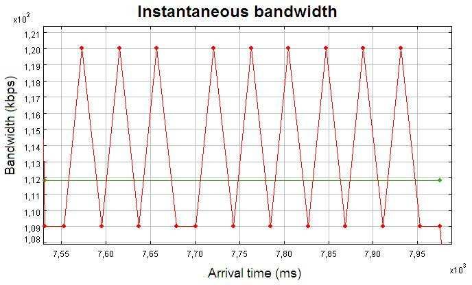
4.     MEASUREMENT METHODOLOGY

4.1    Measurement technique
   In each experiment probe packets are sent at a constant
rate for a short time period. In order to estimate the in-
stantaneous bottleneck link capacity, probe packets must be
enqueued together in the radio access buffer (assuming that
the wireless link is the bottleneck). The packet rate to ac-
complish this is chosen as the maximum mobile capacity
(that depends on the mobile class).
   There is a tradeoff in the selection of the probe packet
size. The accuracy in the analisys of each activity interval
time is important. In order to have more samples in each             Figure 1: Cross traffic effect on bottleneck capacity
activity interval time it is necessary to send packets with          measures.
the smallest size allowed. However, in order to have less
uncertainty in the capacity estimation from the measures of           Multiclass Slot      DL Slots      UL Slots     Active Slots
the inter-arrival times, it is preferred to use as big as possible           1                1             1              2
packet sizes.                                                                2                2             1              3
   The time stamp absolute error is around 1 ms. To solve                    3                2             2              3
this tradeoff packet sizes around 300 − 500 bytes are used.                  ..               ..            ..             ..
These sizes are the smallest that provide a capacity estima-                  .                .             .              .
tion relative error lower than 10% for the biggest GPRS-                     9                3             2              5
EDGE capacities that are around 120 − 240 kbps.                             10                4             2              5
   Next subsection summarizes the most common used method-
ologies for wired link capacity estimation. In subsection 4.3
wireless link capacity estimation problems are explained.            Table 1: Mobile classification by its multiclass slot
                                                                     type.
4.2    Bottleneck link capacity estimation
   For each packet pair the link capacity can be estimated as        4.3     Wireless TDMA systems issues
$
∆t
   ,  where $ is the packets size and ∆t is the inter-arrival
time between consecutive packets at the client. After this           4.3.1    Introduction
estimation, the values obtained for each packet pair are clas-         In general, in cellular networks, the bottleneck is located
sified for further processing. By this processing a final ca-        on the air interface. In addition to the problems explained
pacity is estimated.                                                 before in the case wired link capacity estimation, the follow-
   If a pair of packets (with packet size $) wait together           ing issues arise in the case of cellular wireless links:
in the bottleneck link buffer (with link capacity C), and in
not any other link, the time between arrivals is $     . One            • Mobile class
                                                     C
important issue to point out is that packet pair estimation             • Carrier to interference ( ci ) relation
capacity may be distorted by cross traffic or by limitations
on the measurement system.                                              • Available time slots for data transfer in the serving cell
   There are two situations that may affect the measure-
                                                                     Mobile class
ments. The first situation happens if there is cross traffic
between probe packets. In this case they will be separated a         The mobile class is a classification between different types
time T , which is larger than the separation imposed by the          of terminals which determines how many simultaneous time
bottleneck capacity. In this case the system will estimate           slots can be used by the client in order to transfer data. Ta-
a fake bottleneck capacity C 0 < C. The other situation              ble 1 lists most commonly used class types and the number
happens when the probe packets wait in queues after the              of time slots used for download (DL) and upload (UL) in
bottleneck link. In this case they will join together yield-         each class.
ing a fake bottleneck capacity C 0 > C. These effects are
illustrated in figure 1. These cases must be filtered. The
                                                                     Carrier to interference relation
                                                                                                      ` ´
capacity estimation will be more accurate if the bottleneck          Carrier to interference relation ci is the parameter which
link is not heavy loaded by cross traffic and the last queue         determines the effective rate of data transfer per time slot.
of the path is at the bottleneck link.                               When ci relation is small, the error probability during the
   Several techniques are used for processing packets pairs          transfer is high. In order to avoid this problem, when ci
and estimate the capacity, filtering the cases explained be-         relation is small, more redundancy bits are used. The more
fore. Usually, histogram classification or kernel density es-        redundancy bits are used to transfer information, the less
timation are used. Pathrate [4] and Nettimer [10] use these          is the information rate per time slot. Table 2 list different
techniques.                                                          available code schemes in EDGE (MCS).
   The main idea of these algorithms is to estimate the ca-
pacity by finding the maximum of the distribution (or his-           Available time slots for data transfer
togram). This value represents the estimated capacity that           The service provider configures the number of available time
occurs more frequently.                                              slots for data transfer in the cell. So, some of the configu-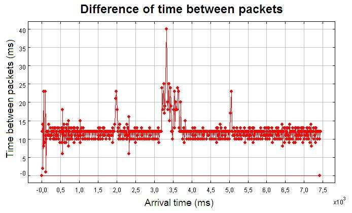
MCS           BW per TS (at layer 2, in kbps)                         demand time slots, and they have priority over data users
         1                         8.8                                        on these channels. In this case the data users can only use
         2                        11.2                                        the fixed data time slots and the on-demand time slots that
         3                        14.8                                        are not used for voice calls. So, the capacity is determined
         ..                         ..                                        by the mobile class, ci relation and on-demand time slots
          .                          .                                        availability (instantaneously determined by the amount of
         8                        54.4                                        voice calls). In this case the link capacity is modulated by
         9                        59.2                                        voice traffic.
                                                                              Number of GSM users are less or equal than fixed voice
     Table 2: Different code schemes in EDGE.                                 slots, the client shares the channel with other data users
                                                                              and a fixed ci relation is assumed.
      Data User 1                                                             In this case the client is sharing data resources with other
                                                                              data users. Thus, each data user does not have the channel
                                                                              for his own use all the time. This case can be seen as a
                                                                              fixed capacity system (assuming a fixed number of users
                                                                              transmitting all the time with a fixed ci relation) shared in
                                                                              time with other data users.
                              C      V     V     D    OD    OD    OD     OD
     Data User N                                                              Number of GSM users are higher than fixed voice slots,
                            C: Control channel                                the client shares the channel with other data users and
                            V: Voice (GSM) channel
                                                                              a fixed ci relation is assumed.
                            D: Data channel                                   This is a more realistic case which can be seen as the super-
  Voice Users (GSM)         OD: On demand channel (between voice and data)    position of the two cases mentioned before. So, in this case
                                                                              the link capacity is modulated by voice traffic and shared in
                                                                              time with other data users.
 Figure 2: Typical GPRS-EDGE queueing system.
                                                                              More complex cases.
                                                                              A more realistic model is obtained by the superposition of
ration variables in the cell are the number of fixed time                     all the above mentioned variables, which includes variation
slots assigned to data transfer, the number of fixed time                     of data and voice traffic and ci relation. Another relevant
slots assigned to voice traffic and the number of on-demand                   effect is cross traffic inserted in the channel by the data client
time slots between voice and data. Usually, for the on-                       (another kind of traffic different from the probe packets that
demand time slots, voice calls has preemptive priority over                   may introduce certain level of noise on it). The following
data transfers.                                                               algorithm deals with this situation.
   Cellular link capacity can not be estimated using the same
procedures as in the wired links case because cellular links                  5.     ALCE: AN ALGORITHM TO ESTIMATE
may have capacity time variations. This problem is analyzed
in more detail in the following subsection.                                          CELLULAR LINK CAPACITY
                                                                               This algorithm is composed by different modules. The
4.3.2 GPRS-EDGE Queueing System                                               main modules are the following:
   Figure 2 shows a typical GPRS-EDGE queueing system.                             1. Activity and inactivity intervals classification
As it can be seen, this system may include interaction be-
tween voice and data users. There are multiple factors that                        2. Analysis of each activity interval
impact on the capacity estimation. In the following para-
                                                                                       A. Potential capacities detection
graphs different situations are analyzed in order of complex-
ity.                                                                                   B. Process of samples for each one of the capacities
                                                                                          detected in A
Number of GSM users are less or equal than fixed voice
slots, there is only one data user in the cell and a fixed                         3. Parameters estimation
c
i
  relation is assumed.                                                        5.1      Activity and inactivity intervals classifica-
In this case, voice users do not use on-demand time slots.                             tion
All data time slots are available for the client. Therefore,                     In order to find the activity intervals, an adaptation of
the client has all data resources available all the time. The                 the K-means algorithm [2] was developed. The algorithm
capacity will be only determined by the mobile class and ci                   calculates K − 1 thresholds and classifies the packet pair
relation. Assuming a fixed ci relation this case is similar to                inter-arrival time into K groups, where K is supposed to be
the classical wired one, like ADSL.                                           known. In our case K = 2 represents the group of samples
                                                                              that belong to one activity interval (group 1) and the group
Number of GSM users are higher than fixed voice slots,                        of samples that denotes a change of activity interval (group
there is only one data user in the cell and a fixed ci                        2). Once the execution of the algorithm is finished, the
relation is assumed.                                                          selected threshold is given by
In this case there are more users than fixed voice slots as-                                                      g1 + g2
signed by the operator. So, voice users need to use on-                                             T hKmeans =                             (5)
                                                                                                                     2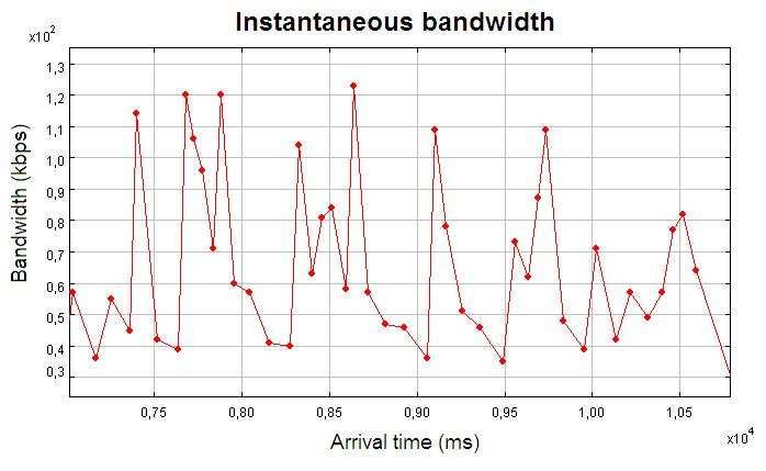
Figure 3: Experiment in which activity intervals are               Figure 4: Experiment in which there is only one
clearly denoted.                                                   activity interval.

where g1 and g2 are the means of the groups 1 and 2 respec-
tively.
   One particular case is when during the experiment does
not occur more than one activity interval. This happens
when the client has the channel for his own use. In this
case, at the moment of distinguishing between activity inter-
vals, if we run the “pure” K-means algorithm, an incorrect
discrimination is done, identifying some differences of time
between consecutive packets as inactivity intervals.
   In order to solve this problem a minimum threshold is
calculated when detecting the intervals. The time between
packet arrivals depends on the packet size and on the in-
stantaneous capacity, so, a minimum threshold, T hmin , is
calculated based on this parameters.
   Applying this criterion, the final threshold applied to dif-
ferentiate between inactivity periods is given by equation
6.
                                                                   Figure 5: “Pure” K-means algorithm finds many fake
              T hm = max {T hmin , T hKmeans }              (6)    inactivity intervals.
Figure 3 shows the situation of a common experiment, in
which activity intervals are clearly denoted and separated
by inactivity intervals. On the other hand, figure 4 shows         the density function f (t) as
an experiment in which there are not any inactivity intervals                                  n    „        «
                                                                                   ˆ        1 X       t − Xi
,so, the adaptation of the K-means algorithm is necessary to                       f (t) =        K                      (7)
                                                                                           nh i=1        h
obtain valid results.
   As an example, if we run the “pure” K-means algorithm,          where K is a kernel function and h is the bandwidth. The
figure 5 shows how a great number of false inactivity inter-       kernel has the following properties
vals are detected.                                                                  Z ∞
                                                                                         K(t)dt = 1, K(t) ≥ 0            (8)
5.2     Activity interval analysis                                                   −∞

  After detecting activity intervals, the algorithm proceeds       The Kernel used in the algorithm is the Epanechnikov Ker-
to analyze each one of them. The flow diagram of this mod-         nel, defined as
ule is shown in figure 6.                                                                         3
                                                                                      K(t) =        (1 − t2 )I|t|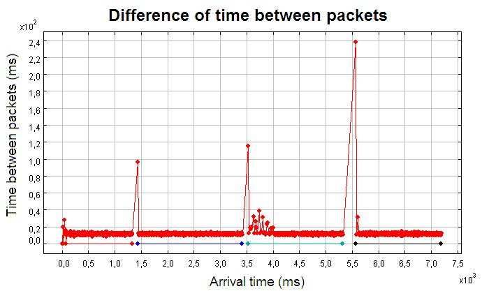
START

                                          NO
                        Are intervals?                 END

                                YES

                                               Remove packets from
                       Density function
                                                these sub intervals
                       of the interval

                      Find maximums of
                         the density
                                                Mark sub intervals
                           function
                                                with this capacity

              NO
                       Are maximums?
                                               Take the maximum of           Figure 7: Capacity detection in presence of low level
                                                greatest bandwidth
                                                     available               of noise.

                                    YES

Figure 6: Flow diagram of the activity interval anal-
ysis.

by the following equation

                   hopt = (40)1/5 π 1/10 sn n−1/5                     (10)
where sn represents the standard deviation of the samples.
                          n
                                       !1/2
                      1X             2
               sn =         (Xi − X)                  (11)
                      n i=1

  After the density function is obtained the algorithm pro-
ceeds to find its maximums, being these points the potential
capacities during the activity interval.

5.2.2    Samples processing to avoid false potential ca-                     Figure 8: Capacity variations due to time stamps
         pacities detected                                                   accuracy.
   In this module, the algorithm evaluates if these potential
capacities really correspond to an activity interval.
   In order to discard false capacities a set of rules are ap-
plied to the potential capacities. For example, rules to avoid               system or measures affected by cross traffic. For these rea-
capacities that are not possible in a cellular wireless link,                sons the algorithm behaves as shown in figure 7.
rules to avoid spurious measurements or rules to take into                      In figure 8 a particular case is shown. In this experiment
account capacity variations due to the limited accuracy of                   the instantaneous link capacity oscillates between 120 and
the measurement procedure can be considered.                                 109 kbps. This situation is probably caused by the accuracy
   At the end of this procedure all valid capacities in the ac-              in the time stamps. Particularly, in this case, the experiment
tivity interval of study are saved. The process is repeated                  was done with a packet size of 300 bytes, while the registered
with the next activity interval until there are no more activ-               inter-arrival time were between 22 and 20 ms. However, it is
ity intervals to analyze. When this module is finished, the                  reasonable to suppose that the packets arrived at the client
algorithm executes the following one.                                        at a rate between 22 and 20 ms. This means that the real
   Figure 7 shows a common situation in the analysis of an                   capacity is between 120 and 109 kbps. It can be seen how,
activity interval. In this case, a great quantity of samples                 by the application of the kernel density estimation, the final
register the same capacity. However, the presence of certain                 capacity is detected at 113 kbps.
isolated samples which are far from this value could induce                     Figure 9 shows a case in which the experiment was done
to think, at first sight, in the presence of many capacities                 under several noise conditions. As it can be seen it is not
during the activity interval. However, due to the rules im-                  easy to find the real link capacity. Under these conditions
posed to filter spurious capacities, the algorithm identifies                the capacity estimation would have large uncertainty, so the
these isolated points as invalid measurements done by the                    algorithm does not mark any capacity.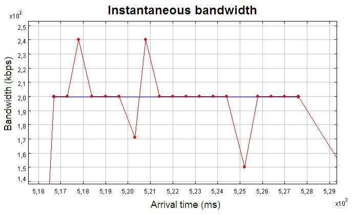
At the beginning of the experiment, its parameters are ne-
                                                                  gotiated between the client (Applet or Midlet) and the server
                                                                  via HTTP packets. After this negotiation, the server begins
                                                                  the experiment by sending UDP probe packets with the cho-
                                                                  sen parameters. Since the initial request for the experiment
                                                                  is done by the client, the edge router register an exchange
                                                                  of HTTP packets from the client (which has a private IP
                                                                  address) to the server (with a public IP address). Once this
                                                                  exchange is finished the server starts sending UDP packets
                                                                  to the client. If the server sends the UDP probe packets to
                                                                  the private client’s IP, the packets will be discarded by the
                                                                  router. If the server sends the probe packets to the edge
                                                                  router public IP, the packets will be discarded, because the
                                                                  router does not know which client has requested these pack-
                                                                  ets.
                                                                     To solve this problem, the system implements the “de-
                                                                  ceive” phase. In this phase the client sends false probe pack-
                                                                  ets to the server immediately after the HTTP negotiation.
Figure 9: Capacity detection with high level of noise.            By doing this, a register on the NAT table of the edge router
The algorithm is not able to distinguish any capac-               associates an UDP flow from the client to the server in any
ity.                                                              given pair of ports. The server reads the information of
                                                                  this UDP packets and starts the experiment by sending the
                                                                  probe UDP packets to the client using the ports chosen by
                                                                  the client in the deceiving phase. In this case, when the ex-
                                                                  periment packets arrive at the edge router, a record on the
                                                                  NAT table exists, so the router knows that this flow belongs
                                                                  to the client - server path and routes the packets correctly.

                                                                  6.2   Phase II: Experiment
                                                                     The experiment sends UDP packets from the server to the
                                                                  client in order to gather the needed information to run the
                                                                  previous algorithm. The packets sent from the server, are
                                                                  rebounded at the client and received by the server. This
                                                                  packets contain useful information for the algorithm as a
                                                                  sequence number and the arrival time stamps at each end
                                                                  of the path.

       Figure 10: Network measurement system.
                                                                  7.    RESULTS
                                                                     During the trial period, many experiments were done un-
                                                                  der different circumstances. The variables taken into ac-
6.     IMPLEMENTED MEASUREMENT SYS-                               count were the place of the experiment (cell of service), ci
       TEM                                                        relation, hour of the day and the mobile type. Experiments
                                                                  were done with two mobiles, Mobile A and Mobile B. Both
   The implemented measurement system consists of a server
                                                                  were used as modems, connected to a PC and using the
running Linux and a Servlet. The client can use an Applet
                                                                  Applet as the client software or as a mobile client, using
(if the client is using a GPRS-EDGE modem) or a Midlet
                                                                  the Midlet as the client software. The places chosen to run
(if the client is using a cellular phone only). Figure 10 shows
                                                                  the experiments were different neighborhoods of Montevideo
a diagram of the measurement system. The system archi-
                                                                  (Punta Carretas, Malvı́n, La Blanqueada and Palermo) and
tecture is explained in more detail in [12].
                                                                  a seaside (Playa Hermosa).
   The measures are done in two phases:
     • Phase I: Edge router deceive                               7.1   Mean capacity
                                                                     Table 3 shows maximum, mean and minimum values of
     • Phase II: Experiment                                       capacities registered during the experiments. Punta Car-
6.1      Phase I: Edge router deceive                             retas, Palermo and Playa Hermosa (P.H.) were the chosen
                                                                  places, and the measures were done using Mobile A.
   The local GPRS-EDGE provider assigns IP addresses to              In these experiments was observed that under normal traf-
its clients from a private pool through an edge router ap-        fic conditions mean capacities were between 190 and 220
plying NAT1 . For this reason, it is necessary to find a way      kbps. These results reveal that Mobile A obtains, in gen-
to establish the communication between the Internet server        eral, four time slots for download with code scheme between
and the client in order to make the corresponding measure-        MCS-6 and MCS-9.
ments. This first phase “deceives” the edge router in order          Figure 11 shows experiments made in Playa Hermosa. In
to establish a path from the server to the client.                this case the pattern of mean capacities on the first three
1
    Network Address Translation                                   days of experiments done in the afternoon were greater than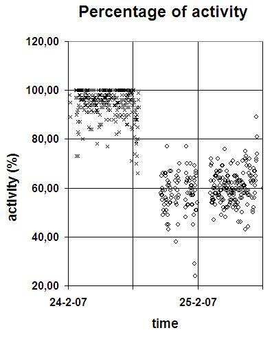
Place of           Mean          Min          Max
        study            capacity     capacity     capacity
                          (kbps)       (kbps)       (kbps)
     P. Carretas            200          167          212
       Palermo              202          187          224
  P.H. - Afternoon          196          142          216
    P.H. - Night            142          115          203

Table 3: Mean capacities registered by place with
Mobile A.

                                                                   Figure 12: Mean capacity with mobile B (cross) and
                                                                   A (circles).

Figure 11: Mean capacity in kbps in Playa Her-
mosa’s cell with Mobile A.

the mean capacities registered at night. This is because the
experiments were done during a holiday weekend in a sea-
side, and at night the voice traffic is more important. Also,
it can be seen that this phenomenon is not appreciated the
last day of the holiday, because the majority of the people
had returned to their residence cities.
                                                                   Figure 13: Mobile B (cross) and Mobile A channel
   Figure 12 shows the capacity obtained with both mobiles
                                                                   (circle) activity time.
in Malvı́n. As it can be seen, mean capacities registered
with mobile B are much smaller than the ones registered
with Mobile A. Doing several experiments in different hours        of traffic on it, as table 5 shows.
and places, the influence of factors like cell of service or the
time of the experiment were discarded; then such behavior          7.4    Jitter
was caused by the type of mobile used.                                From the experiments done we conclude, as expected, that
                                                                   registered jitter is tightly related to RTT.
7.2    Channel Activity time                                          Table 6 shows values obtained in different places. This
  As mentioned in Section 3, channel activity time is an in-       range of values entail that certain services which require low
dicator of the amount of time that the client is using the         jitter values, like Push To Talk, suffer a high degradation of
resources. Figure 13 shows the channel activity time regis-        performance.
tered with both mobiles. As it can be seen, channel activity
time of mobile B was bigger than channel activity time of          7.5    Packets loss
mobile A.                                                            The registered loss in the majority of cases was between
                                                                   0 and 4 % of packets sent. However, in some experiments
7.3    RTT                                                         this ratio was above 10 %.
  After the experiment phase was finished, we concluded
that the delays registered on the network were high in order
to provide real time applications.
  Values obtained with both mobiles were different, as it can
be seen in table 4. Cell of service also have influence over
the RTT obtained, because of the ci relation or the amount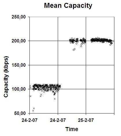
Mobile       Mean           Min            Max                Place of                  Mean             Min            Max
       used       RTT (ms)     RTT (ms)       RTT (ms)                 study           Jitter (ms)      Jitter (ms)       Jitter (ms)
      Mobile A      1329           833           2318              P. Hermosa                  36                22             92
      Mobile B      897            709           1803             P. Carretas                  23                 5             57

Table 4: Registered RTT in Punta Carretas cell with              Table 6: Jitter obtained in different places with mo-
both mobiles.                                                    bile A.

     Place of       Mean            Min            Max
       study       RTT (ms)      RTT (ms)      RTT (ms)
                                                                                   INTERNET
     P. Hermosa      2376            920           8043
                                                                                                     Radio base station
 P. Carretas         1329            833           2318
                                                                                                                           GPRS-EDGE Client

Table 5: RTT obtained in different places with mo-
bile A.
                                                                  FTP Server

8.     THROUGHPUT VS CAPACITY: INFLU-
       ENCE OF THE TRANSPORT LAYER PRO-                                        Figure 14: Measurement topology.
       TOCOL AND THE ROUND TRIP TIME
   The previous section analyzes the cellular link capacity      fer on users terminal (Ethereal) and a software that mon-
and other important performance parameters. The focus of         itors the rate of bits that arrives to the modem (NetStat
this section is on the throughput. The throughput is an          Live). At first, one download was done, studying station-
important parameter at the application layer. Even if the        ary achieved throughput. Then the number of simultane-
system has high capacity, such capacity can not be used          ous downloads was increased, studying again the aggregated
unless a high throughput is acheieved.                           stationary throughput. This procedure was continued until
   Link throughput is an estimator of data transfer rate that    aggregated throughput stop rising.
an application can achieve, whereas capacity refers to the
real “physical” capacity of the access medium. Taking these      8.2     Study of capacity and throughput in up-
considerations into account, the maximum throughput that                 link for different types of traffic
an user could achieve is equal to the link capacity.                In this experiment a tool for capacity estimation was used,
   There are many parameters that influence the through-         Iperf. This tool is based on TCP and UDP traffic in order to
put. The capacity of the bottleneck link is an important         measure real uplink capacity and achieved uplink through-
parameter, but the RTT and the transport layer protocol          put for the client for different kinds of traffic.
have an important influence too.                                    Estimations obtained with this tool depend on the kind
   In our experiments the throughput obtained by a GPRS-         of traffic which is used. In the case that this traffic is UDP,
EDGE connection is in many cases, more than two times            estimation consists in sending one or more bursts of UDP
lower than the bottleneck link capacity. The problem to          flows from the client to the server, flooding the link and an-
analyze is why there is such a big difference. With this pur-    alyzing the packets in the server, as shown in figure 16. In
pose, several measures have been done directly on the net,       case that this traffic is TCP, one or more of TCP connec-
using different kinds of traffic between a server and a mobile   tions are opened, determining aggregated throughput at the
client. Figure 14 shows the topology used on the experi-         server, as shown in figure 17.
ments. The client has a GPRS-EDGE modem, while in
the other side of the communication resides an FTP server,       8.3     Results
from which different file transfers and measurements have
been done.                                                       8.3.1         Study of throughput for TCP traffic in the down-
   All measurements have been done late at night. This pe-                     link
riod was chosen in order to assume a low charge of the cel-        The number of FTP transferences done, in chronological
lular network. ci relation was high enough to ensure that        order, was: 1 file, 2 files, 3 files, 5 files, 1 file, 4 files and
during all the experiments use EDGE channels with high           5 files. Figure 17 shows the achieved throughput for each
MCS. With these assumptions, it is supposed that the client      case.
will achieve high transfer rates.                                  Table 7 shows achieved throughput in the experiment
                                                                 varying the number of FTP transferences.
8.1     Study of throughput for TCP traffic in the                 This experiment shows how the achieved throughput from
        downlink                                                 a single TCP connection did not reach channel capacity.
  In this experiment multiple large files were downloaded,       The link capacity is around 180 kbps, because the mobile
studying achieved throughput by the user (figure 15).            was using 3 slots for download (3+2 configuration). This
  To do such measurements we have used a traffic snif-           case shows that one connection can achieve only a third of
Numb. of FTP Throughput
transferences (kbps)
FTP N
1 58,3
FTP 2 INTERNET 2 96,1
FTP Server
FTP 1
3 135,6
5 161,5
GPRS-EDGE Client 1 64,8
4 146,2
Figure 15: Downlink TCP throughput. 5 158,5
Iperf server
Table 7: Throughput estimation through simultane-
ous FTP downloads.
UDP Flow
Iperf client
INTERNET
Server
traffic and different number of connections/flows.
Number of TCP Estimation
GPRS-EDGE Client connections (kbps)
1 56,3
Figure 16: Uplink throughput.
2 74,2
the link capacity. However, this value could be increased by 3 91,5
opening some simultaneous connections. For five simulta-
neous connections achieved throughput is close to the link
capacity. Table 8: Estimation of uplink capacity with Iperf
It is known that TCP throughput cannot be equal to the using TCP connections.
link capacity because its congestion control algorithm de-
creases the throughput. However, in this case the difference
seems to be important. The problem is that TCP through- Number of UDP flows Estimation
put is inversely proportional to the RTT [13]. As it can be
seen in Table 5, in all cases the RTT is high compared to flows (kbps)
usual values obtained in typical wired links. The RTT is 1 114
normally high in cellular networks and this value generates
the small throughput that can be obtained by one connec- 2 112
tion. 3 117
8.3.2 Study of capacity and throughput in uplink for
different types of traffic Table 9: Estimation of uplink capacity with Iperf
Tables 8 and 9 summarizes estimations for both kinds of using UDP flows.
To analyze the results, it is important to consider the
characteristics of the different kinds of traffic. In the case
of UDP traffic, estimations are equal to the uplink capacity,
independently of the number of flows. In the case of TCP
traffic, all the results obtained were the same as in downlink,
180 only one connection achieved a lower throughput than a few
T = 161,5 kbps
T = 135,6 kbps simultaneous connections.
160
In this sense, capacity estimation using TCP traffic is not
140 recommended. For this reason, it was implemented in the
system end-to-end measurements using UDP packets.
Throughput (kbps)
120
T = 158,5 kbps
100
T = 146,2 kbps 9. CONCLUSIONS
T = 96,1 kbps
80
In this work we have introduced both, an end-to-end mea-
60 surement system and a specific algorithm to measure per-
T = 58,3 kbps T = 64,8 kbps formance parameters in TDMA based IP networks, particu-
40
Figure 17: Downlink throughput during the exper- larly on GPRS-EDGE. This algorithm has the particularity
iment. 20
0 50 100 150 200 250 300
of350being 400
specifically designed for the analysis of the GPRS-
SamplesEDGE protocol, obtaining big amounts of information for [12] J. A. Negreira, J. Pereira, and S. Pérez. MetroCel:
it. Estimación de performance sobre enlaces
Several experiments have been done in order to test the GPRS-EDGE, 2007.
robustness of the system and the algorithm, obtaining good http://iie.fing.edu.uy/˜javierp/MetroCel.
results. Due to this results we have done an extensive mea- [13] J. Padhye, V. Firoiu, D. Towsley, and J. Kurose.
surement on a GPRS-EDGE network, getting to know its Modeling TCP throughput: A simple model and its
main characteristics. empirical validation. Proceedings of the ACM
The developed system can be used through any GPRS- SIGCOMM ’98 conference on applications,
EDGE network. The only requirement is to have a Java technologies, architectures, and protocols for computer
Virtual Machine installed on the client (in case that the communication, pages 303–314, 1998.
client is connected to the GPRS-EDGE network through a [14] F. L. Presti, N. G. Duffield, J. Horowitz, and
modem) or a Java capable mobile. D. Towsley. Multicast-based inference of
network-internal delay distributions. ACM/IEEE
10. ACKNOWLEDGMENTS Transactions on Networking Vol 10, pages 761–775,
2002.
This work was supported by the “Programa de Desarrollo
Tecnologico (PDT)”, project S/C/OP/46/03, “MetroNet II”. [15] V. Ribeiro, R. Riedi, R. Baraniuk, J. N. J., and
The authors would like to thank ANTEL (Administración L. Cotrell. PathChirp: Efficient available bandwidth
Nacional de Telecomunicaciones), and Laura Aspirot for all estimation for network paths. Passive and Active
the support given to the project. Measurement Workshop, 2003.
[16] B. Silverman. Density estimation for stadistics and
data analysis. 1986.
11. REFERENCES [17] J. Strauss, D. Katabi, and F. Kaashoek. A
[1] M. Adler, T. Bu, R. Sitaraman, and D. Towsley. Tree measurement study of available bandwidth estimation
layout for internal network characterizations in tools. Internet Measurement Workshop, Proceedings of
multicast networks. NGC ’01: Proceedings of the Third the 2003 ACM SIGCOMM conference on Internet
International COST264 Workshop on Networked measurement, pages 39–44, 2003.
Group Communication, pages 189–204, 2001. [18] Y. Tsang, M. Coates, and R. Nowak. Network delay
[2] F. Bon. Técnicas no supervisadas. Métodos de tomography. IEEE Transactions on Signal Processing.
agrupamiento. course notes from universidad de Vol. 51, pages 2125–2136, 2003.
granada. 2001. [19] B. A. Turlach. Bandwidth selection in kernel density
[3] R. Cáceres, N. G. Duffield, Horowitz, and D. Towsley. estimation. A review, Discussion Paper 9317, Institut
Multicast-based inference of networkinternal loss de Statistique, Voie du Roman Pays 34, B-1348
characteristics. IEEE Transactions on Information Louvain-la-Neuve, Belgium, 1993.
Theory Vol. 45, pages 2462–2480, 1999.
[4] C. Dovrolis, P. Ramanathan, and D. Moore. What do
packet disperssion techniques measure? Infocom,
pages 905–914, 2001.
[5] A. Downey. Using pathchar to estimate internet link
characteristics. Measurement and Modeling of
Computer Systems, pages 222–223, 1999.
[6] V. Jacobson. Pathchar, a tool to infer characteristics
of internet path. Presented at the mathematical
sciences research institute. 1997.
[7] M. Jain and C. Dovrolis. Pathload: A measurement
tool for end-to-end available bandwidth. Proceedings
of Passive and Active Measurements (PAM), pages
14–25, 2002.
[8] M. Jain and C. Dovrolis. Pathload: A measurement
tool for end-to-end available bandwidth. In
Proceedings of Passive and Active Measurements
(PAM) Workshop, 2002.
[9] M. Jain and C. Dovrolis. End-to-end available
bandwidth: measurement methodology, dynamics, and
relation with TCP throughput. IEEE/ACM
Transactions in Networking, 2003.
[10] K. Lai and M. Baker. Nettimer: A tool for measuring
bottleneck link bandwidth. Proceedings of the
USENIX Symposium on Internet Technologies and
Systems, 2001.
[11] E. Lawrence, G. Michailidis, and V. N. Nair. Inference
of network delay distributions using the EM algorithm.
Technical Report, University of Michigan, 2003.You can also read