2D Rotation-Angle Measurement Utilizing Least Iterative Region Segmentation - MDPI
←
→
Page content transcription
If your browser does not render page correctly, please read the page content below
sensors
Article
2D Rotation-Angle Measurement Utilizing Least
Iterative Region Segmentation
Chenguang Cao           and Qi Ouyang *
 School of Automation, Chongqing University, Chongqing 400044, China; guangcc@foxmail.com
 * Correspondence: yangqi@cqu.edu.cn; Tel.: +86-139-8365-1722

 Received: 3 March 2019; Accepted: 3 April 2019; Published: 5 April 2019

 Abstract: When geometric moments are used to measure the rotation-angle of plane workpieces,
 the same rotation angle would be obtained with dissimilar poses. Such a case would be shown as an
 error in an automatic sorting system. Here, we present an improved rotation-angle measurement
 method based on geometric moments, which is suitable for automatic sorting systems. The method
 can overcome this limitation to obtain accurate results. The accuracy, speed, and generality of this
 method are analyzed in detail. In addition, a rotation-angle measurement error model is established
 to study the effect of camera pose on the rotation-angle measurement accuracy. We find that a
 rotation-angle measurement error will occur with a non-ideal camera pose. Thus, a correction method
 is proposed to increase accuracy and reduce the measurement error caused by camera pose. Finally,
 an automatic sorting system is developed, and experiments are conducted to verify the effectiveness
 of our methods. The experimental results show that the rotation angles are accurately obtained and
 workpieces could be correctly placed by this system.

 Keywords: geometric moments; camera pose; rotation-angle; measurement error

1. Introduction
     An automatic sorting system has the advantages of high efficiency, low error rate, and low labor
cost. It is widely used in several fields, such as vegetable classification [1,2], the postal industry [3],
waste recycling [4,5], and medicine [6]. To meet the requirements of intelligent sorting in industrial
environments, a vision system is often used to sense, observe, and control the sorting process. In this
system, the pose and position of the workpiece are obtained using a camera with image processing,
and the actuator is driven according to these parameters. Consequently, the adaptive ability of the
automatic sorting system will be improved. Generally, pose is described by angles in space [7]. For a
plane workpiece, only one angle is needed. To place a plane workpiece correctly, the rotation angle
of each workpiece must be calculated. Because workpieces are placed arbitrarily in the sorting area,
they should be placed in the storage area in one pose. Therefore, the rotation-angle is an important
parameter that is used to plan a path for the actuator. An incorrect rotation-angle will lead to an error
in path planning, causing the workpieces to be placed incorrectly.
     Rotation-angle measurement is an important component of visual measurement and has been
substantially studied. As a result, various visual rotation-angle measurement methods have emerged,
and they are used in different fields. Existing rotation-angle measurement methods are mainly
classified into four categories. The first one is template matching, in which the rotation angle is
calculated through a similarity measurement. This method is simple, but it has a high computational
cost and is slow. The main challenges for template matching are the reduction of its computational
cost and improvement of its efficiency [8]. The second category is polar transform. The advantage
of this method is that any rotation and scale in Cartesian coordinates are represented as shifts in the
angular and the log-radius directions in log-polar coordinates, respectively [9]. Then, the rotation

Sensors 2019, 19, 1634; doi:10.3390/s19071634                                 www.mdpi.com/journal/sensors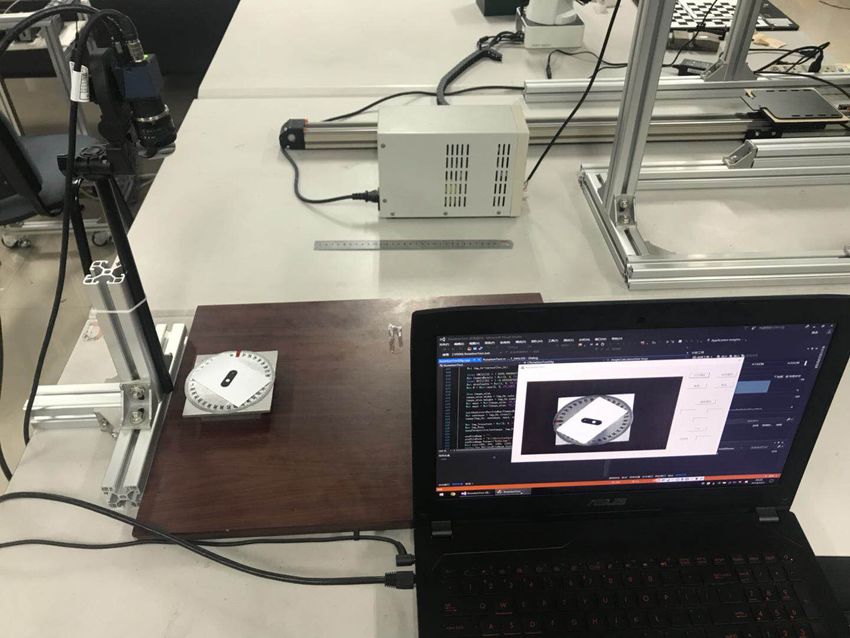
Sensors 2019, 19, 1634                                                                           2 of 17

angle is obtained between two images. The third category of methods takes advantage of the feature
line and feature point in images. The feature line is obtained by Hough transformation or from
the image moment [10]. The angle between the matching lines in two images is calculated, and it
could be regarded as the rotation angle. Such methods are simple and suitable for fast detection.
Feature points are some local features that are extracted from the image. They remain constant
for rotation, scaling, and various types of illumination. Scale-invariant feature transform (SIFT) is
always used to obtain feature points [11], and the rotation angle is calculated by matching points
in different images. In [12], a isosceles triangle is established and then the rotation-angle between
two points could be obtained by solving the triangle formed by origin coordinates and position of
these two points. The fourth category of methods requires auxiliary equipment, which mainly include
a calibration board and projector. In [13], a calibration pattern with a spot array was installed at
the rotor. The rotation angle of the spot array is detected with the equation of coordinate rotation
measurement. The standard deviation of rotation-angle measurement is smaller than 3 arcsec. In [14],
a practical method to measure single-axis rotation angles with conveniently acquirable equipment
was presented. Experiments achieved a measurement accuracy of less than 0.1◦ with a camera and a
printed checkboard. The Moire fringe is an optical phenomenon used in rotation-angle measurement.
The principle of measurement is that the width of the Moire fringe varies as the angle between the
grating lines varies [15]. Lensless digital holographic microscopy is used to accurately measure
ultrasmall rotation angles [16]. Furthermore, white-light interferometry was used in a previous study
to measure one-dimensional rotation angles [17]. In that study, the rotation angle was measured with
an optical plane-parallel plate with a standard refractive index. The phase change of the interference
spectrum of the interferometer was output during the rotation of the plane workpiece.
      It should be noted that although many methods have been developed, these methods are not
suitable for automatic sorting system. This is because the method used in the automatic sorting
system has three requirements. Firstly, the rotation angle needs to be calculated correctly in a short
time. Secondly, auxiliary equipment should not be used, because of the continuous movement of
the workpieces. Thirdly, the method has generality and can calculate the rotation-angle of different
workpieces. Therefore, a new rotation-angle measurement method which satisfies the above conditions
is needed.
      In the present paper, an improved rotation-angle measurement method based on geometric
moments is proposed. The improved method is suitable for workpieces of all shapes and could
overcome a limitation of geometric moments when calculating the rotation-angle. The analysis of speed
and accuracy of the proposed method shows that it can meet the requirements of automatic sorting
systems. In addition, a rotation-angle measurement model is established, and the relationship between
camera pose and rotation-angle measurement error is investigated. Subsequently, a correction method
is presented to reduce the measurement error caused by camera pose. Experimental results show that
this method is accurate and suitable for rotation-angle measurement. The remainder of this paper
is organized as follows. Section 2 reviews the concept of image moment and clarifies the limitation
of rotation-angle measurement based on geometric moments. Section 3 describes the rotation-angle
measurement method in detail. Section 4 establishes a rotation-angle measurement model and
illustrates that a measurement error can be caused by camera pose. Subsequently, a correction method
for rotation-angle measurement error is presented. In Section 5, an automatic sorting system is set up,
and experimental results are discussed. Section 6 draws conclusions.

2. Basic Theory

2.1. Image Moment
      The concept of moments was initially proposed in classical mechanics and statistics. At present,
it is widely used in image recognition [18,19], image segmentation [20], and digital compression [21].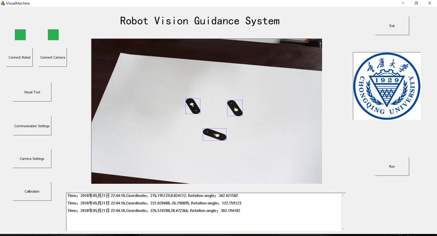
Sensors 2019, 19, 1634 3 of 17
The geometric moment of an image is the simplest, and lower moments have a clear physical meaning
in an image.
Area is expressed by the zeroth moment:
n m
M00 = ∑ ∑ I (i, j). (1)
i =1 j =1
Center of mass is expressed by the first moment:
n m
M10 = ∑ ∑ i · I (i, j)
i =1 j =1
n m
(2)
∑ ∑ j · I (i, j)
M01 =
i =1 j =1
M10 M
xc = , yc = 01 . (3)
M00 M00
The second moments are defined as:
n m
M20 = ∑ ∑ i2 · I (i, j)
i =1 j =1
n m
M02 = ∑ ∑ i · j · I (i, j)
(4)
i =1 j =1
n m
∑ ∑ j2 · I (i, j)
M
11
=
i =1 j =1
Orientation is used to describe how the object lies in the field of view and it could be expressed
by this three second moments:
b
tan 2θ = (5)
a−c
where
M20
a= − xc2
M00
M
b = 11 − xc yc (6)
M00
M
c = 02 − y2c
M00
θ is an angle which is defined by the direction of the axis of least inertia [22]. It is worth noting
that the summation is used in Equations (1), (2) and (4) because we are dealing with discrete images
rather than continuous images.
Higher moments contain details of the image that are relatively more sensitive to noise.
Redundancies will be shown in the operation of a higher moment owing to its nonorthogonality.
Therefore, many new moments [18,21,23] have been proposed.
2.2. Deficiency of Rotation-Angle Measurement Based on Geometric Moments
The rotation-angle measurement method based on geometric moments is advantageous because
of its high accuracy and speed. However, there is a limitation when this method is used, as illustrated
in Figure 1. The figure shows two workpieces S1 and S2 with different poses. Their centers of mass
A1 and A2 are represented by the yellow ∗ symbols, and their axes are represented by green dotted
lines. The angles θ1 and θ2 of the two axes are equal. The object position and pose are expressed by Pob ,
and the angle of its axis is θob .
Sensors 2019, 19, 1634                                                                              4 of 17

       Assuming that the rotation direction is counterclockwise, when S1 and S2 need to be placed into
Pob , the minimum rotating angle around the center of mass is obtained as follows:

                                                 θob − θn + 180◦ , n = 1.
                                             (
                                      rn =                                                              (7)
                                                 θob − θn ,       n = 2.

where r is the rotation angle.
     The difference between r1 and r2 is 180◦ because θ1 is equal to θ2 . S1 and S2 will be rotated by
the same angle if the angle of the axis is regarded as the rotation angle. Therefore, the same rotation
angle is obtained with dissimilar poses, which is an error of the measurement. The reason is that S1
and S2 are non-centrosymmetric about points A1 and A2 , respectively. Thus, for non-centrosymmetric
workpieces, the same rotation-angle would be obtained with dissimilar poses when the geometric
moments are used for rotation-angle measurement. An automatic sorting system using this method is
only suitable for center-symmetrical workpieces. This limitation significantly decreases the generality
of the system.

      Figure 1. Case where the same rotation angle is obtained with dissimilar poses when using image
      geometric moments.

3. Method for Rotation-Angle Measurement
     An improved method is presented here to overcome the limitation described in the previous
section. The method is called the least iterative region segmentation (LIRS) method which consists of
three steps and geometric information is used to overcome the limitation caused by the shape of the
workpiece. The following two points are made before the LIRS method is introduced:

(1)   We assume that the plane workpiece is uniform and the center of mass is located on the workpiece.
(2)   We assume that the optical axis of the camera is perpendicular to the work plane.

      The LIRS method is illustrated in detail below.

3.1. Image Preprocessing
     An image point will be deviated from its ideal position in the presence of lens distortion [24],
resulting in distorted images. Therefore, the calibration is used to improve the accuracy of
rotation-angle measurement [25]. Moreover, the complicated background and the surface texture
of a workpiece will appear as noise in rotation-angle measurement. Therefore, image processing is
required to acquire a superior binary image. Common methods for image processing include denoising,
grayscale, image morphology, and binarization. The image needs to be segmented into several pieces
when more than one workpiece exists because only one workpiece can be handled at a time.
Sensors 2019, 19, 1634                                                                                5 of 17

3.2. Least Iterative Region Segmentation Method
      The coordinates system is established as shown in Figure 2. The red region is a workpiece. Isw
is a regions which is the minimum enclosing rectangle of the workpiece. Isw0 is also a regions which

boundary is violet dotted line. The axis is shown as blue dotted line and the angle of the axis θ is
obtained from Equation (5). The point A is the center of mass which coordinate is ( x, y).

3.2.1. Judgment of Centrosymmetry
     Two steps are required to judge whether the workpiece is centrosymmetric. Firstly, the center of
Isw should be calculated and the region Isw needs to be extended to Isw     0 , if A is not the center of I .
                                                                                                           sd
After extention, the point A is the center of Isd . Secondly, the region Isd rotated by 180◦ is convolved
                                               0                          0

with the original region. The workpiece is centrosymmetric about the center of mass if the result is
greater than a threshold. The angle in the counterclockwise direction between the two axes can be
regarded as the rotation angle. Otherwise, the next step should be carried out.

                                   Figure 2. Schematic of image extension.

     Template matching is always used for recognition. Therefore, this step can be changed to evaluate
whether the template is centrosymmetric. The next step will be performed when the workpiece
matches the asymmetric template. In this manner, the judgment of centrosymmetry will be completed
before the region segmentation, and the efficiency of LIRS will be improved.

3.2.2. Region Segmentation and Identification
      The purpose of this subsection is to find a separation line which divide the workpiece into two
parts with different areas. A new rectangular coordinate system is established with center of mass as
its origin, as shown in Figure 3. Then, a separation line through the origin is drawn as follows:

                                                y − kx = 0,                                              (8)

where k = tan(θ + nα), α is the deviation angle which range is [0◦ , 360◦ ) and n is the iteration number
which initial value is 1.
      After θ and n are assigned, the equation of the separation line would be obtained. Then the
workpiece could be divided into two parts D1 and D2 according to the relationship between the point
and the line. The areas of D1 and D2 are Γ( D1 ) and Γ( D2 ). When the Γ( D1 ) is equal Γ( D2 ), we need
to add 1 to n and divide the workpiece with the new separation line. The iteration will be stopped
until the condition Γ( D1 ) 6= Γ( D2 ) is met. The larger between the two parts is marked as Dl while the
other is marked as Ds . The workpiece must be divided into two regions with different areas by the
separation line because it is non-centrosymmetric about the center of mass.
      To improve the efficiency of division, the threshold method is used. Firstly, the threshold function
B ( P) = y − kx is established and P ( x, y) is a point in the workpiece. The segmentation function is set
Sensors 2019, 19, 1634                                                                                        6 of 17

up as expressed by Equation (9), and P ( x, y) can be assigned to a region according to the polarity of
the thresh function. Therefore, the workpiece is divided into two parts according to the relationship
between the point and the separation line.
                                               (
                                                   B( P) > 0, P ∈ D1
                                                                                                                 (9)
                                                   B( P) > 0, P ∈ D2

      There are two point which need attention:

(1)   The deviation angle needs to be selected reasonably. We should avoid choosing the symmetry axis
      or its perpendicular axis as the separation line because these axes divide a symmetric workpiece
      into two parts with the same area.
(2)   The area of the workpiece will not be exactly equal after the workpiece is rotated at different
      angles because the images captured by the industrial camera have been already discretized by
      a charge-coupled device and a discretization error will always exist. To eliminate the effect
      of discretization on the measurement, a threshold is employed. The areas of Dl and Ds are
      considered equal when the absolute area difference is less than the threshold.

                              Figure 3. Image segmentation with a separation line.

3.2.3. Rotation-Angle Calculation
      After segmentation, a direction vector ~p can be established from ( xl , yl ) to ( xs , ys ), where ( xl , yl )
is the center of mass of Dl and ( xs , ys ) is the center of mass of Ds . The two coordinates are calculated
by Equation (3). The direction vector can be used to calculate the rotation angle because of rotation
invariance. Assuming that a pose is represented by vector ~p = ( xo , yo ), the rotation angle is obtained
by employing:
                                       ~p × ~q            ∆xxo + ∆yy0
                               Θ=               = q
                                       |~p||~q|
                                                     (∆x )2 + (∆y)2 xo2 + y2o
                                                                   p
                                                                                                              (10)
                                           ∆x = xs − xl , ∆y = ys − yl
                                                     Λ = ~p × ~q                                                (11)

                                                    θ = f (Θ, Λ)                                                (12)

where, Θ is a cosine value and the Λ is symbol which polarity is decided by the relationship between ~q
and ~p. f is a function which calculate the rotation-angle based on Θ and the Λ. The value range of θ
is [0◦ , 360◦ ).
      The result of the LIRS method is shown in Figure 4. The green dotted lines are the separation lines
and the blue dotted lines are axes. The red arrows are the direction vectors and the purple arrows are
the object vectors. Although the slopes of the two axes are the same, the direction vectors are different.
Sensors 2019, 19, 1634                                                                               7 of 17

The angle in the counterclockwise direction between two direction vectors could be regarded as the
rotation-angle. The result shows that the LIRS method can effectively measure the rotation-angle of the
workpiece, and it overcomes the limitation of the conventional rotation-angle measurement method
based on geometric moments.

                                       Figure 4. Result of the LIRS method.

3.3. Evaluation of LIRS Method
     Efficiency, accuracy, and application range are the three most important indexes of automatic
sorting systems. They are affected by the performance of the vision algorithm. Therefore, the applicability
of the LIRS method in industrial environments needs to be evaluated. In this section, the accuracy,
speed, and generality of LIRS as well as the image size are analyzed in detail.
     A schematic of the rotation-angle measurement assessment system is shown in Figure 5.
The experimental set up consists of a CCD, a computer, a support, and rotary equipment, which
includes a pedestal and a rotor. A dial is fixed on the surface of the rotor, and the workpiece is placed
on the dial. The workpiece is rotated by the rotor.

                     Figure 5. Schematic of the rotation-angle measurement assessment system.

      The CCD model is MER-200-14GC. It has a 12-mm lens, and its image resolution is 1628 × 1236.
A support with three degrees of freedom is used to adjust the camera pose. For convenience, the camera
optical axis is made perpendicular to the work plane by adjusting the support. A photograph of the
experimental set up is shown in Figure 6.
      The LIRS method is coded in C++ and compiled for 64 bits under Windows 10, and OpenCV 3.2 is
used to process images. The program is executed using an Intel(R) Core(TM)i5-6300HQ CPU running
at 2.30 GHz with 16 GB RAM. The workpiece is rotated from 1◦ to 360◦ in steps of 1◦ . One image is
obtained per rotation, and the first image is regarded as the reference. Subsequently, rotation angles
are calculated between the reference and the other images.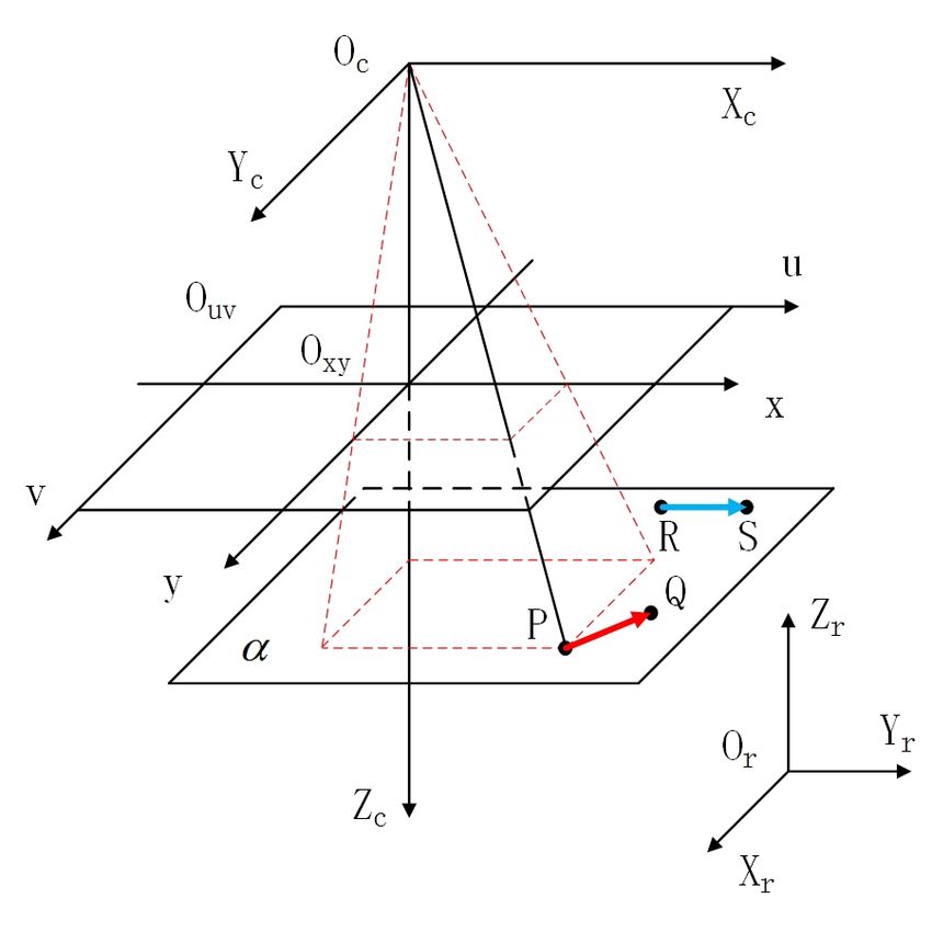
Sensors 2019, 19, 1634                                                                                         8 of 17

                          Figure 6. Experimental set up of the LIRS assessment system.

3.3.1. Accuracy
     The measurement error is shown in Figure 7. The maximum measurement error is less than 0.1◦ ,
which indicates that the LIRS method has a high accuracy. In other words, the LIRS method can be
used to realize rotation-angle measurement with the whole angle range of 1◦ –360◦ in an automatic
sorting system.

                                                         0.15
                              Measurement error/degree

                                                          0.1

                                                         0.05

                                                            0

                                                         -0.05

                                                          -0.1

                                                         -0.15
                                                                 0   60   120     180      240    300   360
                                                                          Rotation-angle/degree

       Figure 7. Measurement error of rotation angle in the experiment when the rotation angle is 1◦ –360◦ .

3.3.2. Time Consumption
      The time consumption of LIRS method is shown in Figure 8. The average time to calculate a
rotation-angle is 62.1136 ms. The time-consumption curve shows large fluctuations because the images
have different sizes. Each image shows the region of interest (ROI), which is determined based on the
minimum external rectangle. The size of the ROI differs after rotation, as shown in Figure 9. Therefore,
the time consumption shows large fluctuations when the whole angle range is measured.

                                                          100

                                                           80
                                           Time/ms

                                                           60

                                                           40

                                                           20

                                                            0
                                                                 0   60   120     180      240    300   360
                                                                          Rotation-angle/degree

         Figure 8. Time consumption of rotation-angle measurement when the rotation angle is 1◦ –360◦ .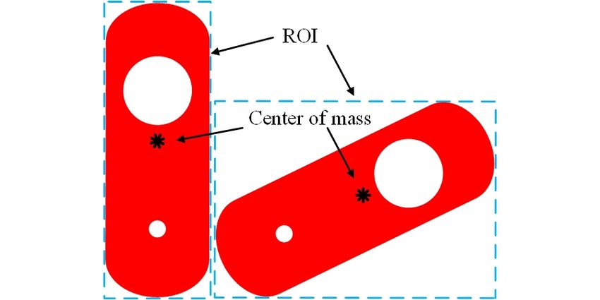
Sensors 2019, 19, 1634                                                                            9 of 17

     There may be several workpieces in an image, and the execution of this program is sequential.
Therefore, the time consumption is high. If the program is run in a field-programmable gate array
(FPGA) device, the parallel-computing features of the FPGA device can be used to reduce the operating
time substantially, further improving the efficiency of the LIRS method.

                     Figure 9. Schematic of ROI selection with the minimum external rectangle.

3.3.3. Generality
     The LIRS method is designed to overcome the limitation of rotation-angle measurement methods
based on geometric moments. The LIRS method has an iteration number n and a deviation angle α,
which can adjust the orientation of the separation line. The LIRS method can find a separation line
for all non-centrosymmetric workpieces. This separation line will be determined uniquely after the
deviation angle is selected. Therefore, the LIRS method has a higher flexibility and a better generality
compared to the conventional method because it is suitable for workpieces of all shapes.

3.3.4. Image Size
      The relationship between the length of the direction vector and the measurement error should be
consider since discretization error exist. Assume that the length of the direction vector is l. Take the
starting point of the vector as the center and draw an one-pixel circle. The maximum directions which
the vector could represent is equal to An , which is also the number of pixels on the circle. Therefore,
with more pixels on the circle, the direction vector can represent more directions. As Figure 10 shows,
L = 70, 130, 180 are selected, and the maximum numbers of angles are An = 636, 792, 1312, respectively.

                                      Figure 10. Schematic of the image size.

     The discretization error between the measured value and the actual value decreases when l is
larger. As the number of direction increases, the discrete values are closer to being continuous values.
Consequently, the accuracy of the LIRS method is increased. For the same workpiece, the length of the
direction vector can be increased by selecting a suitable lens and reducing the distance between the
camera and the workpiece. However, this will increase the size of the ROI and time consumption. It is
necessary to obtain the optimal solution between time consumption and accuracy.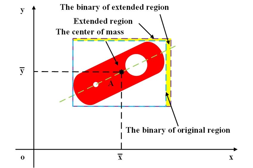
Sensors 2019, 19, 1634 10 of 17
4. Rotation-Angle Measurement Model
4.1. Modeling
When the optical axis is non-perpendicular to the work plane, a dimensional measurement error
will occur. In other words, the accuracy of dimensional measurement is affected by camera pose.
However, the relationship between the accuracy of rotation-angle measurement and camera pose has
not been studied. Therefore, a rotation-angle measurement model needs to be established. Figure 11
shows the basic geometry of the ideal camera model. Three steps are necessary because only an ideal
camera model is addressed [26]. For convenience, the pose in which the optical axis is perpendicular
to the work plane is called the ideal pose. All other camera poses are non-ideal.
Figure 11. Geometry of the ideal camera model.
There are four coordinate systems in this model. The camera coordinate system is composed of
Xc , Yc , and Zc axes and the point Oc . The robot coordinate system is treated as the world coordinate
system, which is composed of Xr , Yr , and Zr axes and the point Or . The pixel coordinate system is
composed of u and v axes and the point Ouv . The image coordinate system is composed of x and y
axes and the point Oxy . The work plane is represented by α. For convenience, we assume that the Zc
axis is perpendicular to the work plane, and the height of the workpiece is neglected. For any point P
in α, its image coordinates can be expressed as Equations (13)–(17).
u f /dx 0 u0 Xc
Zc v = 0 f /dy v0 Yc (13)
1 0 0 1 Zc
Xc Xw tx
Yc = Rz Ry R x Yw − ty , (14)
Zc Zw tz
cos α − sin α 0
R x = sin α cos α 0 , (15)
0 0 1Sensors 2019, 19, 1634 11 of 17
0 0 1
Ry = 0 cos β − sin β , (16)
0 sin β cos β
cos γ 0 − sin γ
Rz = 0 1 0 , (17)
− sin γ 0 cos γ
where f is focal length, dx and dy are the distances between adjacent pixels in the u and v axes,
0
respectively. u0 and v0 are row and column numbers of the center. t x , ty , tz is a translation vector from
the robot coordinate to the camera coordinate system. R x , Ry , and Rz are three rotation matrixes, which
are multiplied in the order of Equation (14). α, β, and γ are three angles. Equation (13) describes the
relationship between camera coordinates system and pixel coordinates system. Equation (14) describes
the relationship between robot coordinate system and camera coordinate system. The equation
of coordinate transformation between pixel coordinate system and the robot coordinate system is
established by using this two equations.
−→
For convenience, vector RS = (1, 0, 0) is considered as the object pose, and the workpiece is
−→ −
→ −→
abstracted as a vector PQ = (∆x, ∆y, 0). RS and PQ are represented by blue and red arrow in
Figure 11, respectly. The work plane in robot coordinates is Zr = Z. The center of mass is treated as
the starting point P, and the center of mass of region Ds is regarded as the ending point Q. Therefore,
−→ −
→
the angle in the counterclockwise direction between PQ and RS can be regarded as the rotation angle.
The ideal value of the rotation angle is
−→ − →
PQ × RS
θi0 = arccos −→ − → , (18)
PQ RS
θi = f θi0 ,
(19)
where f is an adjusting function that makes the value range of the rotation angle [0◦ , 360◦ ).
The measured value is obtained by substituting Equation (13) into Equation (18) and simplifying,
as expressed by Equation (20)
f n1 + ty f n2 1 − c2 + C A f n2 − ty k sin y
θr0 = arccos q q , (20)
0.5 f d12 + f2 f t 2+ f
d2 d3 y d4
θr = f θr0 ,
(21)
where
f n1 = kA sin β − d2 − cos α
b
f n2 = −ty + kt x + tz − Z
b
f n3 = −2ty + kt x + tz −
Z
f d1 = k cos β − B f n2 − D
f d2 = cos α − f n2 sin α
f d3 = 3 − 2 C2 − B2 − cos 2α
(22)
f d4 = 3 − 2 A2 − D2 + cos 2α + 8ty AC
A = sin α cos β
B = cos α sin β
C = cos α cos β
D = sin α sin β
−→
y = kx + b is a line corresponding to PQ in robot coordinates.Sensors 2019, 19, 1634 12 of 17
Thus, the rotation-angle measurement model has been established, and the difference between θi
and θr is the rotation-angle measurement error.
4.2. Simulation and Discussion
It can be seen that the measured value is affected by several parameters, which can be divided
into two categories. The first includes α, β, t x , ty , and the difference between the work plane and
optical center tz − Z. These six parameters will be confirmed after the camera is installed. There
are only two angles in the model, and γ is not included. It can be seen that γ is uncorrelated with
the measured value, and camera rotation around the its optic axis can be neglected in installation.
Thus, camera-installation flexibility is improved in the automatic sorting system. The second category
includes k and b. k is the tangent value of the rotation angle, and b is the position of the vector with
the angle α. When the vector moves along the line, the measured value remains invariant. Otherwise,
it will be changed. This means that different measured values would be obtained for some vectors that
have the same rotation angle but dissimilar positions. This case would result in measurement error.
Figure 12 shows curves of rotation-angle measurement error when four vectors move along the
line y = 50. An approximately linear relationship exists between displacement and measurement
error. The polarity and the rate of error are related to the vectors. This means that different measured
values would be obtained when the workpiece is located at different positions with the same rotation
angle. Figure 13 shows the rotation-angle measurement error in simulation with four values of α and
β. The vector rotates around its starting point in steps of 1◦ . For vectors with different values of α
and β, the measurement-error curves are different. The measured values are different, when the same
vector is selected with different values of α and β. That is, when the same workpiece is measured with
different camera poses, the measured values are different. The polarity and value of the error is related
to the camera pose.
To reduce the rotation-angle measurement error to zero, the following condition should be met:
θi − θr = 0. (23)
Then, Equation (24) will obtained:
α = 0, β = 0. (24)
It can be seen that the measurement error is always present only if the camera is in a non-ideal pose.
10
θ=30 o
Measurement error/degree
8
θ=45 o
6 θ=135o
θ=240o
4
2
0
-2
-4
0 20 40 60 80 100
Displacement of Y axis/mm
Figure 12. Measurement error in the simulation experiment when vectors move along the line y = 50.Sensors 2019, 19, 1634 13 of 17
12
α=10,β=180
Measurement error/degree
α=0,β=190
α=10,β=190
6
0
-6
0 60 120 180 240 300 360
Rotation-angle/degree
Figure 13. Measurement error in the simulation experiment when the vector rotates around its starting point.
4.3. Method for Correction of Rotation-Angle Measurement Error
To meet the condition of perpendicularity, camera should be adjusted by the support before
the measurement. The rotation-angle measurement error will always exist when the camera is in a
non-ideal pose, reducing the accuracy of rotation-angle measurement. To make the measured value
accurate, it is necessary to keep the camera in the ideal pose. In other words, the optical axis needs to
be adjusted to be perpendicular to the work plane. However, this condition cannot be met easily in
industrial environments, because of camera-installation errors or position limitations. The actual pose
could not be coinciding with the ideal pose completely. Therefore, the rotation-angle measurement
error needs to be corrected.
When the camera is in a non-ideal pose, the Zc coordinate of a point on the work plane will be
changed form a constant to a variable. The relationship between the image coordinates and camera
coordinates can be expressed as follows:
X1 Z2 − X2 Z1 Y Z2 − Y2 Z1
∆u = f , ∆v = f 1 , (25)
dxZ1 Z2 dyZ1 Z2
where ( X1 , Y1 , Z1 ) and ( X1 , Y1 , Z1 ) are two camera coordinates in the work plane. dv and du are
∆u 2 + ( ∆v )2 and
p
the
p differences of image coordinates. There is no linear relationship between ( )
( X1 − X2 )2 + (Y1 − Y2 )2 . Therefore, the image will be distorted. This is the primary cause of the
rotation-angle measurement error.
A rotation-angle error measurement correction (REMC) method with an error-correction matrix
is presented to reduce the rotation-angle measurement error. A binary function ω is employed to
multiply with Zc and keep the result constant. A linear relationship will be kept between the image
coordinates and camera coordinates after mapping. The REMC method is illustrated in detail below.
A correction matrix A is introduced as follows:
u0 a11 a12 a13 u
0 1
v = a21 a22 a23 v , (26)
ω
1 a31 a32 a33 1
ω = ua31 + va32 + a33 . (27)Sensors 2019, 19, 1634 14 of 17
The relationship between the image coordinate system (u, v) and camera coordinate system
( Xc , Yc , Zc ) can be expressed as follows:
f Xc f Yc
u= + u0 , u = + v0 . (28)
Zc dx Zc dy
Then, Equation (13) can be rewritten as follows:
u0 F0 0
F12 0
F13 Xw tx
0 11 0 0 0
Zc ω v = F21 F22 F23 Yw − ty , (29)
1 0
F31 0
F32 0
F33 Zw tz
where F is a coefficient matrix and Zc ω can be expressed as
Zc ω = a31 f x Xc + a32 f y Yc + s( a31 u0 + a32 v0 + a33 ). (30)
The work plane in the camera coordinate system can be expressed as follows:
aXc + bYc + cZc − A = 0, (31)
where a, b, c, and A are constant parameters. Three parameters a31 , a32 , and a33 must exist to ensure
the equation holds:
Zc w = A. (32)
Then, (u0 , v0 , 1) can be obtained as follows:
u0 F0 0
F12 0
F13 Xw tx
0 1 11
v = F0 0
F22 0 Y − t .
F23 w y (33)
A 21 0 0 0
1 F31 F32 F33 Zw tz
A is the Zc value of the work plane in the camera coordinate system. It can be seen that the Zc
value can remain invariant during the mapping process. Therefore, the measurement error caused by
camera pose will be reduced when (u0 , v0 ) is used to calculate the rotation angle.
The experimental system is shown in Figure 6. The optical axis is adjusted using the support
to be non-perpendicular to the work plane, and the obtained results are listed in Table 1. It can be
seen that the REMC method can reduce the rotation-angle measurement error caused by a non-ideal
camera pose, and the error is less than 0.1◦ . Therefore, the proposed method is effective and meets
the requirements.
The correction matrix is selected as follows:
4.5985 0.0779219 −1904.15
A = 0.0572827 4.58486 −2660.6 . (34)
2.07701 × 10⁻⁵ 4.75542 × 10⁻⁵ 1
Table 1. Experimental results obtained when the REMC method is employed in the experiment under
a non-ideal camera pose.
Ideal Value Measured Value Correction Value Error
30◦ 31.15◦ 30.11◦ 0.11◦
60◦ 62.95◦ 60.06◦ 0.06◦
120◦ 121.97◦ 119.04◦ 0.04◦
150◦ 150.31.32◦ 150.03◦ 0.03◦
210◦ 210.21◦ 209.09◦ 0.09◦
240◦ 242.61◦ 240.05◦ 0.05◦
310◦ 311.73◦ 319.03◦ 0.03◦
330◦ 330.82◦ 330.06◦ 0.06◦Sensors 2019, 19, 1634 15 of 17
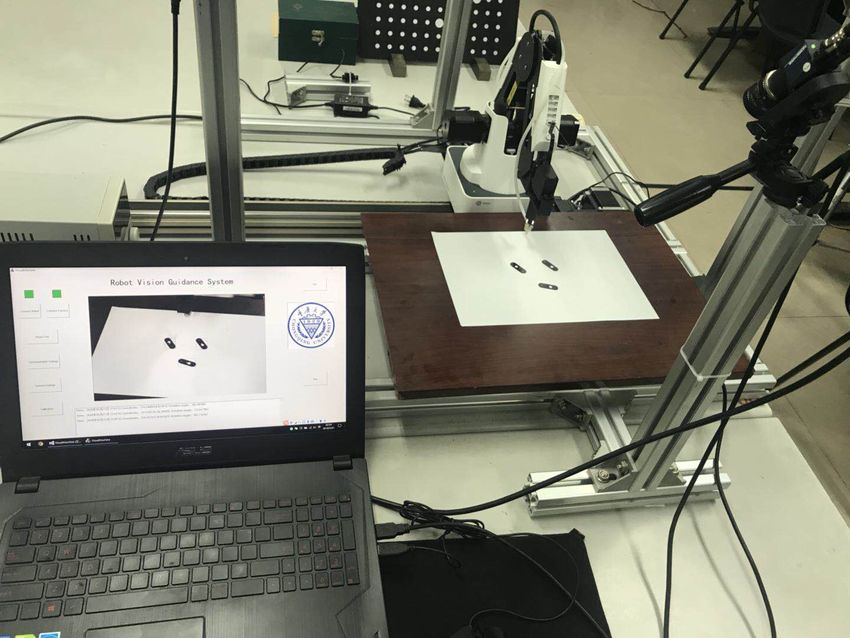
5. Experiment
An automatic sorting system with machine vision is established, as shown in Figure 14. A robot
(Dobot Magician) with a four degrees of freedom robot is used in this system. Four stepping motors
are used to drive a manipulator, which moves with a re-orientation accuracy of 0.2 mm. The software
is coded by MFC with OpenCV 3.2 and consisted of three parts: (1) a camera and a robot control
system including initialization, start and stop functions, and parameter setting; (2) a real-time display
system consisting of an image display and information display; and (3) an information storage system
designed to save important data during program operation. The correction matrix A is selected
as follows:
1.45457 0.383242 −902.439
A = −0.220291 1.86919 −318.915 . (35)
1.57966 × 10⁻⁶ 0.000271224 1
The workpiece is a uniform-thickness thin sheet with two holes of different diameters. The experimental
result is shown in Figure 15. The image with the blue external rectangle and yellow point is shown on
the main interface. Key information is shown in the message region. The results show that the rotation
angles are obtained accurately, and the workpieces could be placed correctly by this system. Therefore,
the LIRS and REMC method could be used in automatic sorting systems in industrial environments.
Figure 14. Automatic sorting system with machine vision.
Figure 15. Result of the experiment.
6. Conclusions
The rotation angle is an important parameter in an automatic sorting system. To accurately
measure the rotation angles of plane workpieces for an automatic sorting system, the LIRS method was
proposed. This method overcomes limitation of the conventional method based on geometric moments,
and it is suitable for workpieces of all shapes. Experimental results show that the measurement error
of the LIRS method is less than 0.1◦ , and the measurement range is between 0◦ and 360◦ . Therefore,Sensors 2019, 19, 1634 16 of 17
the LIRS method meets the requirements of automatic sorting in industrial environments. However, the
average measurement time is approximately 62.1136 ms, which leaves much room for improvement.
A model was established for studying the relationship between camera pose and rotation-angle
measurement error. Then, a formula for calculating the error was derived. The simulation results
show that the measurement error will always exist when the camera is in a non-ideal pose. The value
and polarity of the measurement error are related to the camera pose and location of the workpiece.
Subsequently, the REMC method was designed to correct the rotation-angle measurement error.
The experimental results show that the REMC method is effective, and the measurement error with
the REMC method is less than 0.12◦ .
Finally, an automatic sorting system with the LIRS and REMC method was established, and sorting
experiments were conducted. The two proposed methods yielded accurate rotation angles, and plane
workpieces could be placed correctly by this system.
Author Contributions: Conceptualization, C.C.; methodology, Q.O.; formal analysis, C.C.; software,
C.C.; investigation: C.C.; data curation, C.C.; validation, Q.O.; writing—original draft preparation, C.C.;
writing—review and editing, Q.O.; supervision, Q.O.; project administration, Q.O.
Funding: This work is supported by the National Natural Science Foundation of China (No. 51374264) and
Overseas Returnees Innovation and Entrepreneurship Support Program of Chongqing (No. CX2017004).
Conflicts of Interest: The authors declare no conflict of interest.
References
1. Cho, N.H.; Chang, D.I.; Lee, S.H.; Hwang, H.; Lee, Y.H.; Park, J.R. Development of automatic sorting system
for green pepper using machine vision. J. Biosyst. Eng. 2007, 30, 110–113.
2. Zheng, H.; Lu, H.F.; Zheng, Y.P.; Lou, H.Q.; Chen, C.Q. Automatic sorting of Chinese jujube (Zizyphus jujuba,
Mill. cv. ‘hongxing’) using chlorophyll fluorescence and support vector machine. J. Food Eng. 2010, 101,
402–408. [CrossRef]
3. Basu, S.; Das, N.; Sarkar, R.; Kundu, M.; Nasipuri, M.; Basu, D.K. A novel framework for automatic sorting
of postal documents with multi-script address blocks. Pattern Recognit. 2010, 43, 3507–3521. [CrossRef]
4. Mesina, M.B.; de Jong, T.P.R.; Dalmijn, W.L. Automatic sorting of scrap metals with a combined
electromagnetic and dual energy X-ray transmission sensor. Int. J. Miner. Process. 2007, 82, 222–232.
[CrossRef]
5. Jiu, H.; Thomas, P.; Bian, Z.F. Automatic Sorting of Solid Black Polymer Wastes Based on Visual and Acoustic
Sensors. Energy Procedia 2011, 11, 3141–3150.
6. Wilson, J.R.; Lee, N.Y.; Saechao, A.; Tickle-Degnen, L.; Scheutz, M. Supporting Human Autonomy in a
Robot-Assisted Medication Sorting Task. Int. J. Soc. Robot. 2018, 10, 621–641. [CrossRef]
7. Urizar, M.; Petuya, V.; Amezua, E.; Hernandez, A. Characterizing the configuration space of the 3-SPS-S
spatial orientation parallel manipulator. Meccanica 2014, 49, 1101–1114. [CrossRef]
8. De Saxe, C.; Cebon, D. A Visual Template-Matching Method for Articulation Angle Measurement.
In Proceedings of the IEEE International Conference on Intelligent Transportation Systems, Las Palmas,
Spain, 15–18 September 2015; pp. 626–631.
9. Matungka, R.; Zheng, Y.F.; Ewing, R.L. Image registration using adaptive polar transform. In Proceedings
of the 15th IEEE International Conference on Image Processing, San Diego, CA, USA, 12–15 October 2008;
pp. 2416–2419.
10. Revaud, J.; Lavoue, G.; Baskurt, A. Improving Zernike Moments Comparison for Optimal Similarity and
Rotation Angle Retrieval. IEEE Trans. Pattern Anal. Mach. Intell. 2008, 31, 627–636. [CrossRef]
11. Delponte, E.; Isgro, F.; Odone, F.; Verri, A. SVD-matching using SIFT features. Graph. Models 2006, 68,
415–431. [CrossRef]
12. Munoz-Rodriguez, J.A.; Asundi, A.; Rodriguez-Vera, R. Recognition of a light line pattern by Hu moments
for 3-D reconstruction of a rotated object. Opt. Laser Technol. 2004, 37, 131–138. [CrossRef]
13. Li, W.M.; Jin, J.; Li, X.F.; Li, B. Method of rotation angle measurement in machine vision based on calibration
pattern with spot array. Appl. Opt. 2010, 49, 1001–1006. [CrossRef] [PubMed]Sensors 2019, 19, 1634 17 of 17
14. Dong, H.X.; Fu, Q.; Zhao, X.; Quan, Q.; Zhang, R.F. Practical rotation angle measurement method by
monocular vision. Appl. Opt. 2015, 54, 425–435. [CrossRef]
15. Fang, J.Y.; Qin, S.Q.; Wang, X.S.; Huang, Z.S.; Zheng, J.X. Frequency Domain Analysis of Small Angle
Measurement with Moire Fringe. Acta Photonica Sin. 2010, 39, 709–713. [CrossRef]
16. Wu, Y.M.; Cheng, H.B.; Wen, Y.F. High-precision rotation angle measurement method based on a lensless
digital holographic microscope. Appl. Opt. 2018, 57, 112–118. [CrossRef] [PubMed]
17. Yun, H.G.; Kim, S.H.; Jeong, H.S.; Kim, K.H. Rotation angle measurement based on white-light interferometry
with a standard optical flat. Appl. Opt. 2012, 51, 720–725. [CrossRef] [PubMed]
18. Hu, M.K. Visual pattern recognition by moment invariants. IRE Trans. Inf. Theory 1962, 8, 179–187.
19. Khotanzad, A.; Hong, Y.H. Invariant Image Recognition by Zernike Moments. IEEE Trans. Pattern Anal.
Mach. Intell. 1990, 12, 489–497. [CrossRef]
20. Marin, D.; Aquino, A.; Gegundez-Arias, M.E.; Bravo, J.M. A new supervised method for blood vessel
segmentation in retinal images by using gray-level and moment invariants-based features. IEEE Trans.
Med. Imaging 2011, 30, 146–158. [CrossRef] [PubMed]
21. Mandal, M.K.; Aboulnasr, T.; Panchanathan, S. Image indexing using moments and wavelets. IEEE Trans.
Consum. Electron. 1996, 42, 557–565. [CrossRef]
22. Berthold, K.P.H. Robot Vision; MIT: Boston, MA, USA, 1987; p. 50.
23. Liu, Z.J.; Li, Q.; Xia, Z.W.; Wang, Q. Target recognition of ladar range images using even-order Zernike
moments. Appl. Opt. 2012, 51, 7529–7536. [CrossRef]
24. Ouyang, Q.; Wen, C.; Song, Y.D.; Dong, X.C.; Zhang, X.L. Approach for designing and developing
high-precision integrative systems for strip flatness detection. Appl. Opt. 2015, 54, 8429–8438. [CrossRef]
[PubMed]
25. Munoz-Rodriguez, J.A. Online self-camera orientation based on laser metrology and computer algorithms.
Opt. Commun. 2011, 284, 5601–5612. [CrossRef]
26. Tian, J.D.; Peng, X. Three-dimensional digital imaging based on shifted point-array encoding. Appl. Opt.
2005, 44, 5491–5496. [CrossRef] [PubMed]
c 2019 by the authors. Licensee MDPI, Basel, Switzerland. This article is an open access
article distributed under the terms and conditions of the Creative Commons Attribution
(CC BY) license (http://creativecommons.org/licenses/by/4.0/).You can also read