Extended Geometry and Probability Model for GNSS+ Constellation Performance Evaluation - MDPI
←
→
Page content transcription
If your browser does not render page correctly, please read the page content below
remote sensing
Article
Extended Geometry and Probability Model for
GNSS+ Constellation Performance Evaluation
Lingdong Meng 1,2 , Jiexian Wang 2 , Junping Chen 2,3,4, * , Bin Wang 2 and Yize Zhang 2,5
 1   College of Surveying and Geo-Informatics, Tongji University, Shanghai 200092, China; ldmeng@tongji.edu.cn
 2   Shanghai Astronomical Observatory, Chinese Academy of Sciences, Shanghai 200030, China;
     wangjiexian@tongji.edu.cn (J.W.); binw@shao.ac.cn (B.W.); 13zhyize@tongji.edu.cn (Y.Z.)
 3   School of Astronomy and Space Science, University of Chinese Academy of Sciences, Beijing 100049, China
 4   Shanghai Key Laboratory of Space Navigation and Positioning Techniques, Shanghai 200030, China
 5   Department of Maritime Systems Engineering, Tokyo University of Marine Science and Technology,
     Tokyo 1358533, Japan
 *   Correspondence: junping@shao.ac.cn; Tel.: +86-21-34775363

 Received: 1 July 2020; Accepted: 4 August 2020; Published: 9 August 2020

 Abstract: We proposed an extended geometry and probability model (EGAPM) to analyze the
 performance of various kinds of (Global Navigation Satellite System) GNSS+ constellation design
 scenarios in terms of satellite visibility and dilution of precision (DOP) et al. on global and regional
 scales. Different from conventional methods, requiring real or simulated satellite ephemerides,
 this new model only uses some basic parameters of one satellite constellation. Verified by the
 reference values derived from precise satellite ephemerides, the accuracy of visible satellite visibility
 estimation using EGAPM gets an accuracy better than 0.11 on average. Applying the EGAPM
 to evaluate the geometry distribution quality of the hybrid GNSS+ constellation, where highly
 eccentric orbits (HEO), quasi-zenith orbit (QZO), inclined geosynchronous orbit (IGSO), geostationary
 earth orbit (GEO), medium earth orbit (MEO), and also low earth orbit (LEO) satellites included,
 we analyze the overall performance quantities of different constellation configurations. Results show
 that QZO satellites perform slightly better in the Northern Hemisphere than IGSO satellites. HEO
 satellites can significantly improve constellation geometry distribution quality in the high latitude
 regions. With 5 HEO satellites included in the third-generation BeiDou navigation satellite system
 (BDS-3), the average VDOP (vertical DOP) of the 30◦ N–90◦ N region can be decreased by 16.65%,
 meanwhile satellite visibility can be increased by 38.76%. What is more, the inclusion of the polar LEO
 constellation can significantly improve GNSS service performance. When including with 288 LEO
 satellites, the overall DOPs (GDOP (geometric DOP), HDOP (horizontal DOP), PDOP (position DOP),
 TDOP (time DOP), and VDOP) are decreased by about 40%, and the satellite visibility can be increased
 by 183.99% relative to the Global Positioning System (GPS) constellation.

 Keywords: GNSS+ constellations; highly eccentric orbit; low earth orbit; quasi-zenith orbit;
 dilution of precision; geometry and probability model

1. Introduction
      Global Navigation Satellite System (GNSS) performance can be evaluated from several aspects,
such as satellite signal quality [1,2], the precision of broadcast ephemerides [3–5], the multipath
effect [6,7], convergence speed and precision of positioning [8,9]. Among all of these aspects, the satellite
constellation, which defines the observation geometry distribution of navigation systems [10,11], is of
fundamental importance, especially under the progress of constellation design. Satellite visibility
and dilution of precision (DOP), which reflect the geometry distribution quality of constellations,

Remote Sens. 2020, 12, 2560; doi:10.3390/rs12162560                         www.mdpi.com/journal/remotesensing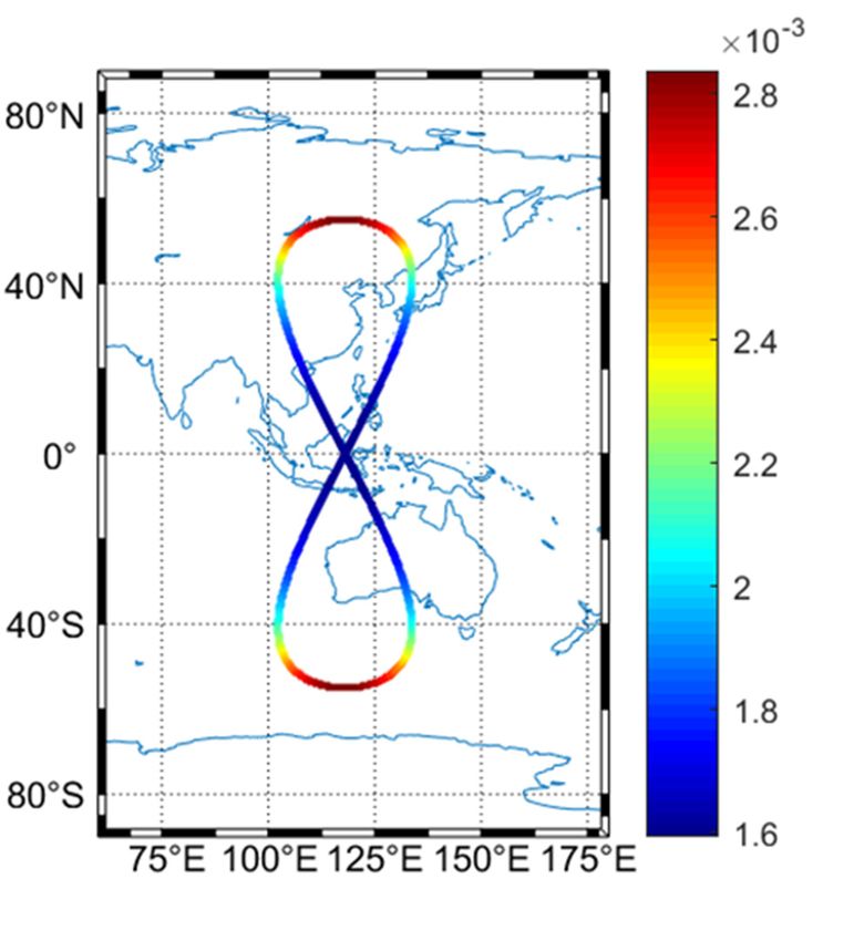
Remote Sens. 2020, 12, 2560                                                                            2 of 21

is regarded as the metric that defines the mapping factor between the ranging error and positioning
error [12,13].
       With the development of the GNSS, the traditional Walker-delta constellation has been transformed
into the hybrid constellation. In order to enhance the service in the area of the Asia-Pacific region
(60◦ S–60◦ N, 50◦ E–170◦ E), the third-generation BeiDou navigation satellite system (BDS-3) constellation
comprises a Walker constellation, inclined geosynchronous orbit (IGSO) constellation, and also the
geostationary earth orbit (GEO) constellation, which dramatically improves the visible satellite number
and DOP in the Asia-Pacific region [14]. Many researchers have analyzed the contribution of IGSO
and GEO constellations for the BDS-3 [2,15].
       However, the DOP of current GNSS constellations in high latitude areas is much larger than
regions of middle and low latitude [15,16], which causes unfavorable positioning, navigation, and
timing (PNT) performance in these areas. Meanwhile, the current coverage of the satellite-based
augment system (SBAS) [17], relies on GEO satellites to broadcast the correction message, also lacks
the continuous coverage of the polar regions. Besides, because the Arctic shipping routes are excepted
to be the shortest and of considerable economic value from the Atlantic Ocean to Pacific Ocean [18],
it is desirable to improve the satellite visibility and geometry distribution quality in high latitude areas,
especially in the Arctic region. Therefore, given the facts mentioned above, highly eccentric orbits
(HEO) satellites could be used [19]. Among these, the Russian Molniya satellites are the most common,
which can be used to provide communication services for polar regions.
       Conventional methods of satellite visibility and DOPs (GDOP (geometric DOP), HDOP (horizontal
DOP), PDOP (position DOP), TDOP (time DOP), and VDOP (vertical DOP) ) assessment are based
on real ephemerides [20] or simulated almanacs [21,22] after complex calculation. Wang et al. [16]
proposed the geometry and probability model (GAPM) for the Global Positioning Satellite System
(GPS) constellation. The GAPM method applies the concept of statistics to satellite visibility analysis
and defines the satellite spatial distribution probability density function based on the satellite angular
velocity. This method only requires some constellation parameters and dramatically reduces the
calculation burden. This method was later used by Chen J. [23] to calculate the GNSS DOP of low earth
orbit (LEO) satellites. However, GAPM is only suitable for the medium earth orbit (MEO) or LEO
constellations, and to evaluate the contributions of IGSO and GEO satellites of BDS-3, Wang et al. [15]
developed the modified GAPM (MGAPM) method. Through the constraint of the domain of a function
to the ground track of IGSO or GEO satellites, MGAPM realizes the extension of GAPM. By revisiting
their method and considering the GNSS+ constellation with possible non-circular HEO and quasi-zenith
orbit (QZO), we present an extended and modified geometry and probability model (EGAPM) with the
capability of analyzing the contribution of large eccentricity satellite orbit constellations to navigation
performance. EGAPM is validated through the satellite visibility and DOP results compared with
that of precise ephemerides of GPS and BDS-3+QZO. Meanwhile, LEO satellites enhancing GNSS
would be one of the promising development trends in the future [24–26]; hence, we also evaluate the
contribution of the polar LEO constellation to navigation. Besides, we assess the performance of the
GNSS+ constellation with 30 BDS-3, 288 LEO, and 5 HEO satellites using the EGAPM and demonstrate
its superiority to BDS-3 and GPS nominal constellations.

2. Methods
     In the previous GAPM method [15,16], the observing sphere was divided into latitudes and
longitudes grids by 1◦ × 1◦ , and the probability of a satellite appearing in one grid can be determined
by its velocity. This probability is regarded as the satellite observing probability, which is the
basis of the estimation of satellite visibility and DOP. For one specific station on the earth ellipsoid,
the number of visible satellites is the sum of probability of the constellation in the observation area of
the station. Furthermore, the satellite probability is regarded as weighting factors in the calculation of
DOPs. Based on the DOPs, the performance and characterization of satellite visibility and geometry
distribution for one GNSS constellation can be further evaluated. It is noted that the opportunities of a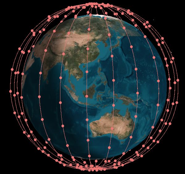
Remote Sens. 2020, 12, 2560 3 of 21
satellite’s appearance in certain areas are zero where the latitude is higher than the satellite’s orbit
incline angle. Because the previous GAPM method is only applicable for the approximately circular
orbit, we modify and extend the GAPM method in this paper to make it applicable for BDS-3 IGSO,
QZO, and HEO satellites.
2.1. MEO and LEO Satellite Observing Probability
For GNSS MEO or LEO satellites in approximately circular orbits, previous GAPM is effective.
The velocity of east-west direction Vλ and north-south direction Vϕ for the position (ϕ,λ) can be written
as [16]: q
cos iorb
Vλ = GM R · r
cos ϕ
cos i 2 , (1)
q
Vϕ = GM
R · 1 − cos orb
ϕ
where GM is the product of the gravitational constant and the earth’s mass; R is the norm of a
satellite position vector; iorb is the satellite’s orbit incline angle to the equator; ϕ is geocentric latitude;
λ is longitude.
As Equation (1) shows, the velocity of satellites appearing in one grid element is a function related
to the latitude. So, for satellites appearing in the grid elements with the same geocentric latitude, the Vϕ
term would be the same. Based on the hypothesis that GNSS satellites are distributed symmetrically in
the east-west direction, the in and out satellites of the grid are balanced in this direction [15]. Therefore,
the observing probability of a satellite depends on Vϕ only. The satellite observing probability can be
modified as [15]: q
k =
R √ k cos ϕ
PM/L = orb , |ϕ| < iorb ,
Vϕ
GM cos2 ϕ−cos2 i
(2)
0, |ϕ| ≥ iorb
where k is the probability constant for a specific GNSS MEO or LEO satellite constellation.
The superscript M/L stands for GNSS MEO or LEO satellites.
As mentioned above, the spherical orbit surface can be divided into 1◦ × 1◦ grids centered in
(ϕi , λ j ):
ϕi = i − 0.5 i = −89, −88, . . . , 90
(
. (3)
λ j = j − 0.5 j = −179, −178, . . . , 180
In addition, the probability constant k can be calculated as [16]:
n
k= , (4)
90 180
P P 1
Vϕ
i=−89 j=−179
where n is the total number of GNSS MEO or LEO satellites.
2.2. GEO and IGSO Satellite Observing Probability
GEO satellites are relatively static to earth in earth-centered earth fixed (ECEF) system. Therefore,
in theory, a GEO satellite will stay at the specific point all the time. For instance, the 3 BDS-3 GEO
satellites are respectively located at 80◦ E, 110.5◦ E, and 140◦ E [27]. So, in theory, the probability of a
GEO satellite appearing at the designed position, such as 80 ◦ E, is 1, while at other arbitrary positions
is 0. Then GEO satellite observing probability can be written as [15]:
(
1, (X, Y, Z) ∈ P
PGEO
(X,Y,Z)
= . (5)
0, other positions
For an IGSO satellite, their satellite ground track is a closed curve. For example, the 3 BDS-3
IGSO satellites, their ground tracks are coincident, while the longitude of the intersection point is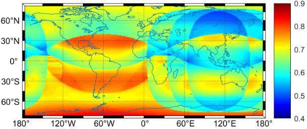
Remote Sens. 2020, 12, 2560 4 of 21
at 118◦ E, with a phase difference of 120◦ [28]. We can calculate a satellite position (X, Y, Z) in the
ECEF system when the true anomaly f turns a specific angle and the set of these points in one earth
self-rotation period is called B in this study. For an IGSO satellite, when f turns over from 0◦ to 360◦ ,
all coordinates in the ECEF system and corresponding velocity in one earth self-rotation period can be
obtained. Considering both the accuracy and computation efficiency, this specific angle can be set at
0.25◦ [15]. Then, refer to the idea of previous GAPM, the probability of IGSO satellites appearing at one
point of B can be determined by the corresponding velocity. So, the modified probability definition,
PIGSO
(X,Y,Z)
, of IGSO satellites to be observed at one point of B can be written as:
IGSO
k
VIGSO , (X, Y, Z) ∈ B
PIGSO
(X,Y,Z)
=
(X,Y,Z) , (6)
0, other positions
where V(IGSO
X,Y,Z)
is the velocity at one point of B in the ECEF system; kIGSO is the probability constant for
IGSO satellites which can be calculated by the following equation:
nIGSO
kIGSO = P 1
, (7)
V IGSO
(X,Y,Z)∈B (X,Y,Z)
where nIGSO is the total number of IGSO satellites with the same ground track. V(IGSO
X,Y,Z)
at one point of B
can be calculated as follows. Firstly, a satellite position (X, Y, Z) in ECEF can be computed with the
true anomaly f as the independent variable. Then, the velocity of X, Y, and Z components: VX , VY , and
VZ can be written as: X ∆t −Xt
VX = t+∆t
Yt+∆t −Yt
VY = , (8)
∆t
V = Zt+∆t −Zt
Z ∆t
where t is one specific epoch; X, Y, and Z are the ECEF coordinates of a satellite at the epoch t or t + ∆t;
∆t means the time elapsed from one point to another very adjacent point. Then, V(X,Y,Z) at one point is:
q
V(IGSO
X,Y,Z)
= 2 + V2 + V2 .
VX Y Z
(9)
We investigate the observing probability of the three BDS-3 IGSO satellites using the modified
observing probability definition of IGSO satellites. From Figure 1, it can be seen that the observing
probability is larger at the northern and southern ends of the figure-8-shape track which is closer to the
actual situation than the corresponding results presented in [15].
2.3. HEO and QZO Satellite Observing Probability
As mentioned above, LEO, MEO, GEO, and IGSO satellites are all in approximately circle orbits
with small eccentricity, and the magnitude of satellites’ position vector and flight velocity vector are
almost constant, which is the prerequisites for the earlier GAPM [15,16]. However, some special
kinds of orbits have larger eccentricity, such as the QZO satellites of the Quasi-Zenith Satellite System
(QZSS) [29]. The eccentricity of QZO satellites of about 0.075 is much larger than that of GPS satellites,
which is normally less than 0.01. To investigate the performance of satellite orbits with large eccentricity,
the traditional GAPM mentioned above should be generalized. For this purpose, the key issue is to
calculate their space coordinates and corresponding velocity in the ECEF system. Therefore, some
points need to be considered: (1) the magnitude of satellite position vector will change all the time;
(2) the time that satellite fly from one point to another adjacent point is different because the satellite
velocity and the magnitude of position vector are changing all the time; (3) the magnitude of satellite
velocity in the ECEF system is changing also.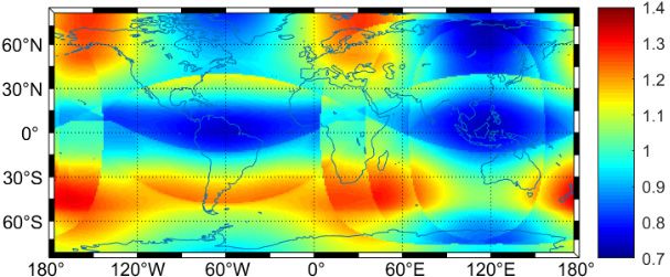
Remote Sens. 2020, 12, 2560 5 of 21
Remote Sens. 2020, 12, x FOR PEER REVIEW 5 of 22
Figure 1. Distribution of observing probability for three third-generation BeiDou navigation satellite
system (BDS-3)
Figure inclined geosynchronous
1. Distribution orbit (IGSO)
of observing probability satellites.
for three third-generation BeiDou navigation satellite
system (BDS-3) inclined geosynchronous orbit (IGSO) satellites.
For point (1), the magnitude of satellite position vector R can be calculated by the following
equation
2.3. HEO [19]:
and QZO Satellite Observing Probability
a 1 − e2
As mentioned above, LEO, MEO, GEO, R = and IGSO satellites, are all in approximately circle orbits
(10)
1 + e cos f
with small eccentricity, and the magnitude of satellites’ position vector and flight velocity vector are
where
almoste isconstant,
the orbitwhich
eccentricity; a is semi-major
is the prerequisites axis.
for the FromGAPM
earlier Equation (10),However,
[15,16]. we knowsomethat the R is kinds
special the
function of the true anomaly f.
of orbits have larger eccentricity, such as the QZO satellites of the Quasi-Zenith Satellite System
For point
(QZSS) (2), according
[29]. The eccentricity to of
Kepler’s
QZO second law, the radius vector sweeps over equal areas in equal
. satellites of about 0.075 is much larger than that of GPS satellites,
time intervals
which [19], i.e.,less
is normally the area
thanrate
0.01.A,To
is ainvestigate
constant: the performance of satellite orbits with large
eccentricity, the traditional GAPM mentioned p above should be generalized. For this purpose, the key
issue is to calculate their space coordinates
. aGM and e2 )
(1 −corresponding velocity in the ECEF system.
A= . (11)
2
Therefore, some points need to be considered: (1) the magnitude of satellite position vector will
change all thethe
Therefore, time; (2) thetime
elapsed timefor
that
thesatellite
satellitefly
fromfrom oneone point
point to to another
adjacent adjacent
point can bepoint is different
calculated by
.
because the satellite velocity and the magnitude of position vector are changing
the equation, A/A, where A is the area that radius vector swept during the period. If the true anomaly all the time; (3) the
magnitude
changes by a of satellite
very smallvelocity
amountin thethe
and ECEF areasystem
that the is changing
radius swept also.could be regarded as a circular
sector, then the area of this tiny circular sector, dA, can be calculatedcan
For point (1), the magnitude of satellite position vector R by be
thecalculated by the following
following equation:
equation [19]:
2
1a(1a−1e −) e
2 2
1 2
dA = R d fR== d f , (12)
(10)
2 21 + 1e +
cose cos
f f
,
where
where df eisisthe
thetiny
orbit eccentricity;
change a is semi-major
of true anomaly. The whole axis.area
From couldEquation (10),
then be we know
derived that
by the the
area R is the
integral
function
within of the true
the interval + 0.25◦ ]:f.
[f, fanomaly
For point (2), according to Kepler’s second law, the radius vector sweeps over equal areas in
2
, is
◦
equal time intervals [19], i.e., the area1ratef +A
Z 0.25 1 − e2
a aconstant:
A= d f . (13)
1 + e cos2 f
2 f
aGM (1 − e )
=
A (11)
However, the analytical expression of this integration 2 is quite . complex, and the result of numerical
integration can be used. The interval [f, f + 0.25◦ ] is divided into 10,000 pieces, and the above equation
Therefore, the elapsed time for the satellite from one point to adjacent point can be calculated by
can be reformulated as:
the equation, A / A , where A is the area that radius vector swept during the period. If the true
anomaly changes by a very small amount and the area that the radius swept could be regarded as a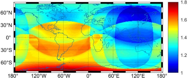
Remote Sens. 2020, 12, 2560 6 of 21
2
10000
1 X a 1 − e2
A≈ (0.000025i). (14)
2 1 + e cos( f + 0.000025i)
i=1
Thus, the elapsed time, ∆t, can be written as:
A
∆t ≈ . . (15)
A
When ∆t is determined, satellite velocity in the ECEF system could be derived. Satellite coordinates
in the orbital plane coordinate system can be written as:
η f = R cos f
(
, f = 0, 0.25, . . . , 360, . . . ., (16)
ξ f = R sin f
where η is the axis points to the ascending node and ξ is the axis points to the direction on the argument
of the latitude of 90◦ .
Satellite coordinates can be transformed from the orbital plane coordinate system into the
ECEF system:
ηi
Xi
Yi = R3 (−Ωi )R1 (−iorb ) ξi ,
(17)
Zi 0
where R3 (−Ωi ) and R1 (−iorb ) are rotation matrices as follows:
cos Ωi − sin Ωi
0
R3 (−Ωi ) = sin Ωi cos Ωi
0 ,
(18)
0 0 1
1 0 0
R1 (−iorb ) = 0 cos iorb − sin iorb ,
(19)
0 sin iorb cos iorb
where Ωi is the right ascension of ascending node which can be written as:
π
Ωi = (Ω0 − ∆t · ωearth ) ◦, (20)
180
where Ω0 is the right ascending node at the initial epoch; ωearth is the angular velocity of the earth
rotation. ∆t can be obtained by Equation (15). Thus, all ECEF cartesian coordinates in one earth
rotation period can be calculated and the set of these coordinates is defined as Γ.
As for point (3), the magnitude of satellite velocity in the ECEF system can be calculated using the
Equations (8) and (9).
Finally, the observing probability of a satellite at one point of Γ can be written as:
HEO/QZO
VHEO/QZO , (X, Y, Z) ∈ Γ
k
HEO/QZO
P(X,Y,Z) =
(X,Y,Z) , (21)
0, other positions
where the superscript HEO/QZO stands for HEO or QZO satellites; kHEO/QZO is the corresponding
probability constant for HEO or QZO satellites of large eccentricity orbits with the same ground track,
which can be written as:
nHEO/QZO
kHEO/QZO = P 1
, (22)
HEO/QZO
(X,Y,Z)∈Γ V(X,Y,Z)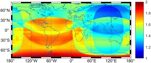
probability constant for HEO or QZO satellites of large eccentricity orbits with the same ground track,
which can be written as:
n HEO / QZO
k HEO / QZO =
1
Remote Sens. 2020, 12, 2560 V HEO / QZO
(22)
7 of 21
( X ,Y , Z )∈Γ ( X ,Y , Z )
,
HEO/QZO HEO/QZO
wherennHEO
where / QZO is the
is the total
total number
number ofof HEO
HEO oror QZOsatellites
QZO satelliteswith
withthe
thesame
sameground track; V(HEO
groundtrack; X,Y,Z)
/ QZO
( X ,Y , Z )
is the velocity of HEO or QZO at one point of Γ in the ECEF system.
is the velocity of HEO or QZO at one point of Γ in the ECEF system.
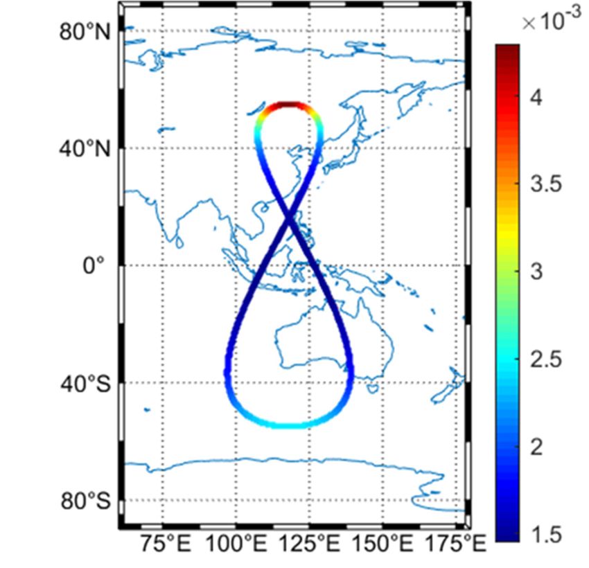
Based on the mentioned above, observing the probability distribution of 3 QZO satellites can
Based on the mentioned above, observing the probability distribution of 3 QZO satellites can be
be seen from Figure 2. The eccentricity of QZO is set as 0.075, but the inclination and the center of
seen from Figure 2. The eccentricity of QZO is set as 0.075, but the inclination and the center of the
the longitude of the ground track are the same as IGSO of BDS-3. The distribution shows that the
longitude of the ground track are the same as IGSO of BDS-3. The distribution shows that the
probability is larger at the northern end of the track, which is very different from IGSO satellites, as a
probability is larger at the northern end of the track, which is very different from IGSO satellites, as
consequence of the velocity near apogee being lower.
a consequence of the velocity near apogee being lower.
Figure 2. Distribution of observing probability for three Quasi-Zenith orbit (QZO) satellites.
Figure 2. Distribution of observing probability for three Quasi-Zenith orbit (QZO) satellites.
2.4. Calculation of DOPs and Satellite Visibility
2.4. Calculation of DOPs and Satellite Visibility
A satellite is visible when it is above a specific cutoff elevation angle (CEA). In this paper, to ensure
A satellite
higher is visible
accuracy, when
we apply theit5◦isCEA
aboveforathe
specific cutoffDOP
following elevation angle (CEA).
and satellite Incalculations
visibility this paper, to
[15].
ensure higher accuracy, we apply the 5° CEA for the following DOP and satellite
We calculated the probability for each satellite that the satellite elevation angle is higher than CEA for visibility
calculations [15]. We Then
each grid element. calculated the probability
the visible for each
satellite number satellite
N can that the
be written as:satellite elevation angle is
higher than CEA for each grid element. Then the visible satellite number N can be written as:
90 180 90 180 90 180
PMEO PLEO PHEO
P P P P P P
N= ij
+ ij
+ ij
+
i=−89 j=−179 i=−89 j=−179 i=−89 j=−179
90 180 90 180 90 180 . (23)
QZO
PIGSO GEO + P
P P P P P
ij
+ P ij
P ij
i=−89 j=−179 i=−89 j=−179 i=−89 j=−179
The observation equation of a satellite can be written as [27]:
δX
δY
v = ex e y ez 1 − l, (24)
δZ
cδt
where ex , ey , and ez are the unit vectors of station-to-satellite vector; v is the residual; cδt the receiver
clock correction; l is the vector of observations; δX, δY, and δZ are the corrections to a station’s
approximate coordinates. In EGAPM, observation equations can be established for each grid or point
higher than specific CEA and corresponding probability is regarded as its weight. Then, using the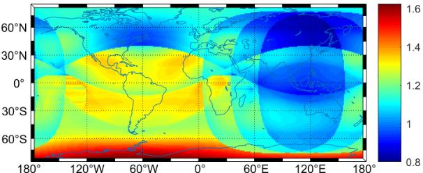
Remote Sens. 2020, 12, 2560 8 of 21
above information, for an arbitrary station on the earth ellipsoid, the coefficient matrix of the normal
equations can be written as [16]:
90 180 90 180 90 180 90 180
P P e2 |
P P P P P P P
Pi j ex e y |D Pi j ex ez |D Pi j ex |D
i=−89 j=−179 i j x D
i=−89 j=−179 i=−89 j=−179 i=−89 j=−179
90 180 90 180 90 180
Pi j e2y |D
P P P P P P
Pi j e y ez |D Pi j e y |D
i=−89 j=−179 i=−89 j=−179 i=−89 j=−179
Nbb = 90 180 90 180
,
(25)
Pi j e2x |D
P P P P
Pi j ez |D
i=−89 j=−179 i=−89 j=−179
90
P 180
P
symmetry Pi j |D
i=−89 j=−179
where D is the visible area above CEA.
The inverse of the normal equation in Equation (25) gives the variance/covariance matrix Q:
−1
Q = Nbb . (26)
Then, the geometric dilution of precision, GDOP, by definition, is the square root of the trace of
the variance/covariance matrix Q.
Cartesian coordinates can be translated into the station’s topocentric up (U), north (N), and east (E)
coordinate system using the following equations:
δX
δU
δU
∂ X Y Z
δY 0 δE δE
δZ = = S
∂ U E N , (27)
δN δN
0 1 cδt
cδt cδt
∂ X Y Z
= R2 (–B)R3 (L), (28)
∂ U E N
where R3 (−L) and R2 (B) are rotation matrices which can be written as follow:
cos(L) sin(L) 0
R3 (L) = − sin(L) cos(L) 0 ,
(29)
0 0 1
cos(−B) 0 − sin(−B)
R2 (−B) = 0 1 0 .
(30)
sin(−B) 0 cos(−B)
Then, the normal equation can be written as:
T
NBLh = S NS. (31)
In addition, the covariance matrix QUEN can be derived using the variance propagation rule as:
T –1
QUEN = S NS . (32)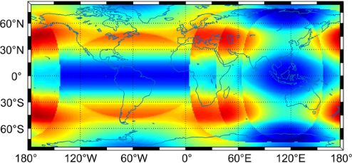
Remote Sens. 2020, 12, 2560 9 of 21
So, by definition, the DOPs can be written as:
p
PDOP = QUEN (1, 1) + QUEN (2, 2) + QUEN (3, 3) position DOP
p
HDOP = QUEN (2, 2) + QUEN (3, 3) horizontal DOP
p
VDOP = pQUEN (1, 1) vertical DOP
TDOP = QUEN (4, 4) time DOP . (33)
q
NDOP = QUEN (3, 3) north DOP
p
EDOP = QUEN (2, 2) east DOP
Obtained from the above expression, the correlation, ρUclk , of station geodetic height between
receiver clock difference follows the expression of:
QBUEN (1, 4)
ρUclk = p p . (34)
QUEN (1, 1) QUEN (4, 4)
In addition, the ratio, NE, of the positioning precision in the longitude component to the latitude
component can be written as:
p
QUEN (3, 3)
NE = p . (35)
QUEN (2, 2)
In summary, we can establish an observation equation based on all grids or points above CEA,
and the probability of satellites in this grid is regarded as the weight of this observation equation. Then,
the normal equation of the GNSS+ constellation can be given by:
GNSS+ MEO LEO GEO IGSO HEO QZO
Nbb = Nbb + Nbb + Nbb + Nbb + Nbb + Nbb , (36)
MEO , N LEO , N GEO , N IGSO , N QZO HEO can be given by Equation (25).
where Nbb bb bb bb bb
, and Nbb
3. Method Validation
We used 24 h averages on global scales of the values derived from real GPS precise ephemerides
provided by GeoForschungsZentrum Potsdam (GFZ) and the precise ephemerides of the BDS-3+QZO
simulation constellation, to validate the usefulness EGAPM and assess the method of satellite visibility
and DOPs estimation. Constellation parameters of BDS-3+QZO and GPS are shown in Table 1.
Table 1. Constellation parameters of third-generation BeiDou navigation satellite system (BDS-3)+
Quasi-Zenith orbit (QZO) and Global Positioning System (GPS) [28–30].
Parameter BDS-3+QZO GPS
Orbit Type MEO QZO GEO MEO
Nominal Number 24 3 3 32
Inclination 55◦ 55◦ 0◦ 55◦
Altitude (KM) 21,528 38,950.6 (Apogee) 35,786 20,200
Period(s) 46,404 86,170.5 86,170.5 43,080
Estimations of the number of visible satellites and corresponding reference values at 5◦ CEA
are shown in Figure 3. Using EGAPM, the root mean squares (RMS) between the estimated and
reference number of visible satellites are 0.10 for 32 GPS satellites and 0.05 for 30 BDS-3+QZO satellites.
Generally, the discrepancies between estimated and reference values at high latitudes are larger than
other locations.
The underestimating rates for the GPS and BDS-3+QZO constellation are calculated (Table 2),
to assess the DOPs underestimation with a 5◦ CEA. The average underestimating rates are 7.95–11.07%.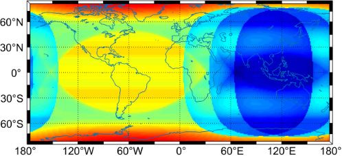
Altitude (KM)      21,528    38,950.6 (Apogee)     35,786    20,200
                                   Period(s)        46,404         86,170.5        86,170.5   43,080

              Estimations of the number of visible satellites and corresponding reference values at 5° CEA are
         shown in Figure 3. Using EGAPM, the root mean squares (RMS) between the estimated and reference
Remote Sens. 2020, 12,
         number    of 2560
                       visible satellites are 0.10 for 32 GPS satellites and 0.05 for 30 BDS-3+QZO satellites. 10 of 21
         Generally, the discrepancies between estimated and reference values at high latitudes are larger than
         other locations.

             Figure
     Figure 3.       3. Estimation
                Estimation    and and  reference
                                   reference       valueofofthe
                                                value        the number
                                                                 number ofofvisible satellites
                                                                              visible          for 32for
                                                                                       satellites      Global Positioning
                                                                                                         32 Global   Positioning
             System (GPS) satellites and the BDS-3+QZO constellation at all latitudes (−90° S–90°        N) for the cutoff
     System (GPS) satellites and the BDS-3+QZO constellation at all latitudes (−90◦ S–90◦ N) for the cutoff
             elevation angle (CEA) ◦of 5°. (a) Estimation and reference value of the number of visible satellites for
     elevation  angle (CEA) of 5 . (a) Estimation and reference value of the number of visible satellites for
             32 GPS satellites; (b) Estimation and reference value of the numbers of visible satellites for BDS-
     32 GPS 3+QZO.
             satellites; (b) Estimation and reference value of the numbers of visible satellites for BDS-3+QZO.

               Average,
     Table 2.The        minimal, and
                 underestimating ratesmaximal   underestimating
                                       for the GPS and BDS-3+QZOrates of the estimated
                                                                   constellation         GPS and
                                                                                  are calculated   BDS-3+QZO
                                                                                                 (Table 2), to
     DOPs   ((GDOP   (geometric DOP),   HDOP    (horizontal DOP), PDOP    (position  DOP),  TDOP    (time DOP),
       assess the DOPs underestimation with a 5° CEA. The average underestimating rates are 7.95–11.07%.
     and VDOP (vertical DOP) )) relative to the reference values ((reference-estimation)/reference × 100%)
     over latitudes.

                                                           Underestimating Rates of DOPs (%)
               Constellation
                                                                  Average (Min–Max)
                                        GDOP                   PDOP                  HDOP                    VDOP
                   GPS             10.41 (5.06–13.10)    9.85 (4.58–12.40)      7.98 (3.96–10.63)      10.33 (4.64–13.03)
                BDS-3+QZO          10.94 (6.93–16.12)    10.39 (6.46–15.09)     7.95 (4.44–10.55)      11.07 (6.79–16.91)

4. Experimental Results and Analyses
      In this section, the satellite visibility and geometry distribution quality of GNSS and GNSS+
constellations are investigated. Firstly, the performance of BDS-3 and GPS is compared. Then, 3 IGSO
satellites of BDS-3 are replaced by 3 QZO satellites and positioning precision of IGSO and QZO satellites
are compared. After that, 5 HEO satellites are combined with BDS-3 to establish the BDS-3+HEO
constellation and the contribution of HEO is investigated. Finally, the performance of the GNSS+
constellation of GNSS+HEO+LEO is assessed.

4.1. BDS-3 VS GPS
     Using the EGAPM the performance of the BDS-3 and GPS constellations is analyzed from
the aspects of satellite visibility, DOPs, correlations level between station height and receiver clock
difference, and the ratio of positioning precision of longitude and latitude components. The results are
shown in Figure 4 and Table 3.
GNSS+ constellation of GNSS+HEO+LEO is assessed.
4.1. BDS-3 VS GPS
Using the EGAPM the performance of the BDS-3 and GPS constellations is analyzed from the
aspects of satellite visibility, DOPs, correlations level between station height and receiver clock
Remotedifference,
Sens. 2020, 12,
and2560 11 of 21
the ratio of positioning precision of longitude and latitude components. The results
are shown in Figure 4 and Table 3.
(a) (b)
(c) (d)
(e) (f)
Remote Sens. 2020, 12, x FOR PEER REVIEW 12 of 22
(g) (h)
(i) (j)
(k) (l)
(m) (n)
(o) (p)
Figure
Figure 4. Estimated
4. Estimated DOPs
DOPs (GDOP(geometric
(GDOP (geometric DOP),
DOP),HDOP
HDOP(horizontal DOP),
(horizontal PDOP
DOP), (position
PDOP DOP),DOP),
(position
TDOPTDOP
(time(time
DOP),DOP),
andand VDOP
VDOP (vertical
(vertical DOP)
DOP) ), positioningprecision
), positioning precisionin
inlongitude
longitude versus
versus latitude,
latitude, and
and correlation between station height and receiver clock difference of the BDS-3 and GPS
constellation with 5° CEA. (a) Number of visible satellites BDS-3; (b) Number of visible satellites GPS;
(c) GDOP of BDS-3; (d) GDOP of GPS; (e) HDOP of BDS-3; (f) HDOP of GPS; (g) PDOP of BDS-3; (h)
PDOP of GPS; (i) TDOP of BDS-3; (j) TDOP of GPS; (k) VDOP of BDS-3; (l) VDOP of GPS; (m) The
ratio of positioning precision between the longitude component and the latitude component of BDS-
3; (n) The ratio of positioning precision between the longitude component and the latitude component
of GPS; (o) Correlation level between station height and receiver clock difference of BDS-3; (p)Remote Sens. 2020, 12, 2560 12 of 21
correlation between station height and receiver clock difference of the BDS-3 and GPS constellation
with 5◦ CEA. (a) Number of visible satellites BDS-3; (b) Number of visible satellites GPS; (c) GDOP
of BDS-3; (d) GDOP of GPS; (e) HDOP of BDS-3; (f) HDOP of GPS; (g) PDOP of BDS-3; (h) PDOP
of GPS; (i) TDOP of BDS-3; (j) TDOP of GPS; (k) VDOP of BDS-3; (l) VDOP of GPS; (m) The ratio of
positioning precision between the longitude component and the latitude component of BDS-3; (n) The
ratio of positioning precision between the longitude component and the latitude component of GPS;
(o) Correlation level between station height and receiver clock difference of BDS-3; (p) Correlation level
between station height and receiver clock difference of GPS.
Table 3. The average, minimal, and maximal visible satellites and DOPs of BDS-3 and GPS.
Average (Min–Max)
Constellation
VisiNum HDOP PDOP TDOP VDOP
BDS-3 in augmentation area 13.20 (11.27–14.86) 0.73 (0.66–0.80) 1.46 (1.31–1.61) 0.67 (0.56–0.74) 1.08 (0.98–1.21)
BDS-3 on global scale 10.48 (7.69–14.86) 0.78 (0.66–0.93) 1.68 (1.31–1.98) 0.73 (0.54–0.84) 1.29 (0.98–1.63)
GPS on global scale 10.99 (10.8–11.75) 0.75 (0.68–0.81) 1.61 (1.51–1.86) 0.69 (0.64–0.78) 1.24 (1.12–1.54)
From Figure 4a,b, we can find that the satellite visibility of GPS is more globally balanced than
BDS-3, and for BDS-3, more satellites can be observed in the Asia-Pacific region while fewer satellites
in the Western Hemisphere. From Figure 4c to Figure 4l, the DOPs of BDS-3 are larger than GPS in
the Western Hemisphere. Note that VDOP is larger in high latitude regions, especially in the polar
regions for both BDS-3 and GPS because, with an increase in station latitude, the elevation of satellites
observed becomes lower. In this case, introducing HEO satellites into the GNSS constellation may
make more satellites be observed, which might improve the geometry distribution in the vertical
direction. As shown in Figure 4m,n, for the GPS constellation in most regions, the positioning precision
in the longitude component is worse than for the latitude component. However, in contrast, for the
BDS-3 constellation in some low latitude regions and some polar regions, the precision of the longitude
component is better. The reason may be that GPS satellites are all MEO satellites, mainly flying along
east-west direction so positioning precision is better in this direction. However, in the case of BDS-3,
3 IGSO satellites mainly fly along the longitude direction. Besides, the GEO satellites mainly contribute
to DOP value in the longitude direction mainly [2]. For the correlation level between station height
and receiver clock difference, as shown in Figure 4o,p, BDS-3 in augmentation area (60◦ S–60◦ N and
50◦ E–170◦ E) is slightly higher than GPS in the same area. This may be because IGSO and GEO fly
slowly and will persist over a user receiver for a longer time. Table 3 shows the average, minimal, and
maximal visible satellite number and DOPs on global and regional scales. In the regional augmentation
area, for BDS-3, 13.2 satellites can be seen on average, 2.7 and 2.2 more than the BDS-3 and GPS global
average, respectively. Similarly, BDS-3 DOPs in the regional augmentation area is more favorable than
BDS-3 and GPS on global scales. Because of fewer operational satellites of BDS-3 than GPS, on a global
scale, visible satellites number and DOPs are slightly worse than GPS.
4.2. BDS-3+QZO Constellation
The QZSS with a service area covering the Asia-Pacific region is an augmentation system for GPS
and Galileo [31]. The QZO satellites of QZSS are similar to the IGSO satellites of BDS-3. They all follow
a figure-8-shape track on the spherical orbit surface in the ECEF system, but QZO satellite’s ground
track is not symmetric for the northern and southern hemisphere. This is because the eccentricity of
QZO is 0.075 and therefore satellites with a higher elevation angle can be more easily observed in urban
areas of Japan, which can improve the geometry distribution in the complex urban environment [32].
The specific parameters of QZO are listed in Table 4.Remote Sens. 2020, 12, 2560 13 of 21
Table 4. Quasi-Zenith orbit (QZO) parameters [29].
Orbit Parameter Nominal Value
Semi-major axis 42,165 km
Eccentricity 0.075
Inclination 41◦
Argument of perigee 270◦
Center of longitude 139◦ East
We replace 3 IGSO satellites of BDS-3 by 3 QZO satellites to investigate the differences between
IGSO and QZO in terms of satellite visibility and GDOP. The inclination is set as 55◦ and the center
of longitude is modified as 118◦ E which is the same as of BDS-3 IGSO satellites. The ground track
of QZO satellites is shown in Figure 2. The values of the BDS-3+QZO constellation parameters are
shown in Table 1.
As revealed by Figure 5, after replacing 3 IGSO satellites, the performance in high latitude regions
of the Northern Hemisphere is slightly improved but in some regions is slightly worse compared to
BDS-3. This is because QZO is in an elliptical orbit and its apogee is in the Northern Hemisphere
Remote Sens. 2020, 12, x FOR PEER REVIEW 14 of 22
leading to QZO satellites spend about 2.3 h longer in the North Hemisphere.
(a) (b)
Figure5.5.The
Figure Theperformance
performanceimproving
improvingrates rates(%)
(%)ofofBDS-3+QZO
BDS-3+QZOrelative
relativetotothe
theBDS-3
BDS-3constellation
constellationinin
area ◦ S–90
areaofof9090° ◦ NN
S–90° and
and ◦ E–170
5050° ◦ E. E.
E–170° (a)(a) Satellites
Satellites visibility
visibility improving
improving ratesrates of BDS-3+QZO
of BDS-3+QZO relative
relative to
BDS-3; (b) GDOP
to BDS-3; improving
(b) GDOP ratesrates
improving of BDS-3+QZO
of BDS-3+QZO relative to BDS-3
relative to BDS-3
4.3.
4.3.BDS-3+HEO
BDS-3+HEOConstellation
Constellation
Although
Althoughthe the hybrid constellation isisapplied
hybrid constellation appliedininBDSBDS and
and QZSSQZSS to improve
to improve the visibility
the visibility in
in some
some specific areas, the visibility in polar regions is still unfavorable. This is because
specific areas, the visibility in polar regions is still unfavorable. This is because that, for the current that, for the
current GNSS constellations,
GNSS constellations, when thewhen the station
station is at higher
is at higher latitudes,
latitudes, the elevation
the elevation of satellites
of satellites that canthatbe
can be observed
observed is lower.
is lower. If satellites
If satellites thatthat
cancan cover
cover highlatitude
high latituderegions
regionsareare included
included in in the
theGNSS+
GNSS+
constellation,
constellation, the geometric distribution for such regions will be improved. The HEO satellites,for
the geometric distribution for such regions will be improved. The HEO satellites, for
example, the Russian Molniya satellites, are the kind of satellites that can fulfill this
example, the Russian Molniya satellites, are the kind of satellites that can fulfill this function [19]. function [19].
These
Thesesatellites
satelliteshave
have synchronous
synchronous 1212h orbits of of
h orbits 500–40,000
500–40,000 kmkmaltitude thatthat
altitude are are
inclined at an
inclined atangle of
an angle
63.4 ◦ to the equator which can not only ensure an exceptional coverage of the Northern Hemisphere
of 63.4° to the equator which can not only ensure an exceptional coverage of the Northern
but also minimizes
Hemisphere but alsotheminimizes
impact of the
orbital perturbations
impact caused by the
of orbital perturbations earth’s
caused byoblateness. The HEO
the earth’s oblateness.
The HEO satellite’s parameters applied in this study are listed in Table 5 and their ground track is
continuously repeated as shown in Figure 6. The HEO in the 3D graphic view is displayed in Figure
7.
Table 5. Highly eccentric orbitsHEO) parameters.
Orbit Parameter Nominal ValueRemote Sens. 2020, 12, 2560 14 of 21
satellite’s parameters applied in this study are listed in Table 5 and their ground track is continuously
repeated as shown in Figure 6. The HEO in the 3D graphic view is displayed in Figure 7.
Table 5. Highly eccentric orbits (HEO) parameters.
Orbit Parameter Nominal Value
Semi-major axis 42,165 km
Eccentricity 0.740969
Inclination 63.4◦
Argument of perigee 270◦
Center of longitude 118◦ E
Remote
Remote Sens.
Sens. 2020,
2020, 12,
12, xx FOR
FOR PEER
PEER REVIEW
REVIEW 15
15 of
of 22
22
Figure 6. Ground
Figure 6. track of
Ground track of highly
highly eccentric
eccentric orbits
orbits (HEO)
(HEO) satellites.
satellites.
Figure 7.
7. HEO
Figure 7.
Figure HEO in
HEO in the
in the three-dimensional
the three-dimensional (3D)
three-dimensional (3D) graphic
(3D) view.
graphic view.
graphic view.
Five HEO
Five HEO satellites
satellites and BDS-3 satellites are combined to
and BDS-3 to establish the BDS-3+HEO
BDS-3+HEO constellation.
constellation.
primary constellation
The primary
The constellation parameters
parameters are
are listed
listed in
in Table
Table6.6.
Table
Table6.6.Parameters
Table Parameters of
6.Parameters of the BDS-3+HEO
BDS-3+HEO constellation.
the BDS-3+HEO constellation.
Parameter
Parameter BDS-3+HEO
BDS-3+HEO
Parameter BDS-3+HEO
Orbit
Orbit Type
Type MEO
MEO IGSO
IGSO GEO
GEO HEO
HEO
Orbit Type MEO IGSO GEO HEO
Nominal
Nominal Number
Number 24
24 33 33 55
Nominal Number 24 3 3 5
Inclination Inclination
Inclination 55◦ 55° 55° 55°
55°55◦ 0°
0° 0◦ 63.4°
63.4° 63.4◦
Altitude (km)
Altitude (km)21,52821,528
Altitude (km) 21,528 35,786 35,786
35,786
35,786 500–40,000
500–40,000 500–40,000
35,786 35,786
Period(s) Period(s)
Period(s) 46,40446,404
46,404 86,170.5
86,170.5
86,170.5 86,170.5
86,170.586,170.5
43,061
43,061 43,061
We evaluate the performance of the BDS-3+HEO constellation on a global scale, as illustrated in
Figure 8.Remote Sens. 2020, 12, 2560 15 of 21
We evaluate the performance of the BDS-3+HEO constellation on a global scale, as illustrated in
Remote Sens. 2020, 12, x FOR PEER REVIEW 16 of 22
Figure 8.
(a) (b)
(c) (d)
(e) (f)
(g) (h)
Figure8.8.Estimated
Figure EstimatedDOPs, DOPs,positioning
positioningprecision
precisionininlongitude
longitudeversus
versuslatitude,
latitude,and
andthethecorrelation
correlation
betweenstation
between stationheight
heightand
andreceiver
receiver clock
clock difference
difference ofofthethe BDS-3+HEOconstellation.
BDS-3+HEO constellation.(a)(a)Number
Numberofof
visiblesatellites;
visible satellites;(b)
(b)GDOP;
GDOP;(c)(c)HDOP;
HDOP;(d) (d)PDOP;
PDOP;(e)(e)TDOP;
TDOP;(f)(f)VDOP;
VDOP;(g) (g)The
Theratio
ratioofofpositioning
positioning
precision
precision between
between the the longitude
longitude component
component and theand the latitude
latitude component;
component; (h) Correlation
(h) Correlation level
level between
between
station station
height andheight
receiverand receiver
clock clock difference.
difference.
The ◦ ◦
Thedetailed
detailedimprovement
improvementrates ratesofofintroducing
introducingHEO HEOsatellites
satellitesrelative
relativetotoBDS-3
BDS-3atat3030°N–90
N–90°NN
region
regionare
aresummarized
summarizedininTable Table7.7.AsAscan
canbebeseen
seenfrom
fromFigure
Figure8 8and
andTable
Table7,7,the
theDOPs
DOPsand andsatellite
satellite
visibility are modified favorably after using 5 HEO satellites. In the 30 ◦ N–90◦ N region, the satellite
visibility are modified favorably after using 5 HEO satellites. In the 30° N–90° N region, the satellite
visibility is improved
visibility is improved on average by 38.76%.
on average In addition,
by 38.76%. all kinds of
In addition, allDOPs
kindsare ofimproved.
DOPs areByimproved.
introducing By
five HEO satellites
introducing to BDS-3,
five HEO on to
satellites average,
BDS-3,values of thevalues
on average, GDOP, ofPDOP, HDOP,
the GDOP, VDOP,
PDOP, and TDOP
HDOP, VDOP,are and
reduced
TDOP by are15.70%,
reduced 16.65%, 10.35%,
by 15.70%, 16.65%,10.35%,
16.65%, and 11.52% respectively.
16.65%, and 11.52% However, the correlation
respectively. However, levelthe
between station
correlation height
level and receiver
between stationclock difference
height is still higher.
and receiver As shown is
clock difference in still
Figure 8h, theAs
higher. correlation
shown in
level in low
Figure latitude
8h, the and thelevel
correlation polar
in region is slightly
low latitude and higher.
the polar What is more,
region as revealed
is slightly higher. in Figures
What 8g
is more,
and 9, after applying HEO satellites, in some regions such as north polar and
as revealed in Figure 8g and Figure 9, after applying HEO satellites, in some regions such as north low latitude regions,
positioning
polar and precision
low latitudein longitude
regions, is better thanprecision
positioning in the latitude component.
in longitude This may
is better than bein since IGSO
the latitude
and HEO satellites mainly fly along the north-south direction, which would
component. This may be since IGSO and HEO satellites mainly fly along the north-south direction, contribute to the DOP
value
whichin would
the longitude component
contribute to the DOPmainly.
value in the longitude component mainly.Remote Sens. 2020, 12, 2560 16 of 21
Remote Sens. 2020, 12, x FOR PEER REVIEW 17 of 22
Table 7. Improvement rates (%) of introducing HEO satellites relative to BDS-3 at 30◦
N region.N–90◦
Table 7. Improvement rates (%) of introducing HEO satellites relative to BDS-3 at 30° N–90° N region.
Average (Min–Max)
Average (Min–Max)
VisiNum GDOP PDOP HDOP VDOP TDOP
VisiNum GDOP PDOP HDOP VDOP TDOP
38.76 38.76 15.70
15.70 16.65
16.65 10.35
10.35 16.65
16.65 11.5211.52
(17.31–50.88) (2.30–23.25) (2.65–24.96) (4.04–18.68) (2.65–24.96) (0–22.73)
(17.31–50.88) (2.30–23.25) (2.65–24.96) (4.04–18.68) (2.65–24.96) (0–22.73)
Remote Sens. 2020, 12, x FOR PEER REVIEW 17 of 22
Table 7. Improvement rates (%) of introducing HEO satellites relative to BDS-3 at 30° N–90° N region.
Average (Min–Max)
VisiNum GDOP PDOP HDOP VDOP TDOP
38.76 15.70 16.65 10.35 16.65 11.52
Figure 9. The
The ratio of positioning precision between the longitude component and the component
(17.31–50.88) (2.30–23.25) (2.65–24.96) (4.04–18.68) (2.65–24.96) (0–22.73)
latitude for BDS-3.
4.4. BDS-3+LEO+HEO
4.4. BDS-3+LEO+HEOConstellation
Constellation
The augmentation
The augmentation of GNSS with
of GNSS with LEO
LEO satellites
satellites is
is one
one of
of the
the most
most interesting
interesting trends
trends inin the
thefuture.
future.
We
We consider the addition of 288 LEO satellites in polar orbits which is mentioned in Li et al. [25] to
consider the addition of 288 LEO satellites in polar orbits which is mentioned in Li et al. [25] to
form the BDS-3+LEO+HEO constellation. The primary constellation parameters are
form the BDS-3+LEO+HEO constellation. The primary constellation parameters are listed in Table 8. listed in Table 8.
These LEO orbits are distributed in 12 planes and orbit altitudes of 1000 km as shown
These LEO orbits are distributed in 12 planes and orbit altitudes of 1000 km as shown in Figure 10 in in Figure 10 in
the 3D
the 3D graphic
graphic view.
view. Using
Using thethe EGAPM,
EGAPM, the theperformance
performanceof ofthetheBDS-3+LEO+HEO
BDS-3+LEO+HEO constellation
constellation is is
analyzed.Figure
analyzed. The results
The results are plotted
9. The ratio
are plotted in Figure
Figure
of positioning
in 11. between the longitude component and the component
precision
11.
latitude for BDS-3.
Table 8. Parameters of the BDS-3+ low earth orbit (LEO)+HEO constellation.
4.4. BDS-3+LEO+HEO Constellation
Parameter BDS-3+LEO+HEO
The augmentation of GNSS with LEO satellites is one of the most interesting trends in the future.
Orbit Type
We consider MEO
the addition of 288 IGSO
LEO satellites GEO
in polar orbits LEO in Li et al.
which is mentioned HEO[25] to
Nominal Number 24 3 3 288 5
form the BDS-3+LEO+HEO constellation. The primary constellation parameters are listed in Table 8.
Inclination 55◦ 55◦ 0◦ 90◦ 63.4◦
These LEO orbits are distributed in 12 planes and orbit altitudes of 1000 km as shown in Figure 10 in
Altitude (km) 21,528 35,786 35,786 1000 500–40,000
the 3D graphic
Period(s)view. Using the EGAPM, the
46,404 performance86,170.5
86,170.5 of the BDS-3+LEO+HEO
6307 constellation
43,061 is
analyzed. The results are plotted in Figure 11.
Figure 10. Low earth orbit (LEO) satellites in the 3D graphic view.
Table 8. Parameters of the BDS-3+ low earth orbit (LEO)+HEO constellation.
Parameter BDS-3+LEO+HEO
Orbit Type MEO IGSO GEO LEO HEO
Nominal Number 24 3 3 288 5
Inclination
Figure
55° 55° 0° 90° 63.4°
Figure 10.10.
LowLowearth
earthorbit
orbit (LEO)
(LEO) satellites
satellitesininthe
the3D3D
graphic view.
graphic view.
Altitude (km) 21,528 35,786 35,786 1000 500–40,000
Period(s)
Table 8. Parameters of 46,404
the BDS-3+ 86,170.5
low earth 86,170.5 6307 constellation.
orbit (LEO)+HEO 43,061
Parameter BDS-3+LEO+HEO
Orbit Type MEO IGSO GEO LEO HEO
Nominal Number 24 3 3 288 5
Inclination 55° 55° 0° 90° 63.4°
Altitude (km) 21,528 35,786 35,786 1000 500–40,000Remote Sens.
Remote 2020,
Sens. 12,12,
2020, x FOR
2560 PEER REVIEW 17 18 of 22
of 21
(a) (b)
(c) (d)
(e) (f)
(g) (h)
Figure
Figure11.11.
Estimated
EstimatedDOPs,
DOPs,positioning
positioningprecision
precision in longitude versusininlatitude,
longitude versus latitude,and
andthethe correlation
correlation
between station height and receiver clock difference of the BDS-3+LEO+HEO
between station height and receiver clock difference of the BDS-3+LEO+HEO constellation constellation with
with 5◦ 5°
CEA.
CEA. (a)(a) Numberofofvisible
Number visiblesatellites;
satellites;(b)
(b)GDOP;
GDOP; (c)
(c) HDOP;
HDOP; (d)(d)PDOP;
PDOP;(e) (e)TDOP;
TDOP;(f)(f)VDOP;
VDOP; (g)(g)
The The
ratio of positioning precision between the longitude component and the latitude component;
ratio of positioning precision between the longitude component and the latitude component; (h) The (h) The
correlation
correlation levelbetween
level betweenstation
stationheight
height and
and receiver
receiver clock
clockdifference.
difference.
As can be seen in Figure 11, after introducing the LEO satellites, the DOPs have decreased
As can be seen in Figure 11, after introducing the LEO satellites, the DOPs have decreased
significantly, which means that the geometric distribution has been improved. Since all LEO satellites
significantly, which means that the geometric distribution has been improved. Since all LEO satellites
are in polar orbits, a lot more satellites can be observed in high latitude regions than in the middle and
are in polar orbits, a lot more satellites can be observed in high latitude regions than in the middle
low latitude areas (Figure 11a). Although hundreds of LEO satellites in polar orbits are introduced, the
and low latitude
correlation betweenareas (Figure
station height11a). Although
and receiver hundreds
clock differenceofis LEO satellites
still higher in 11h).
(Figure polarAsorbits
for theare
introduced,
positioningthe correlation
precision ratiobetween
between station heightand
the longitude andlatitude,
receiverillustrated
clock difference
in Figureis11g,
still Figure
higher9,(Figure
and
11h). As for the positioning precision ratio between the longitude and latitude,
Figure 8g. We can find that LEO satellites mainly contribute to longitude component performance.illustrated in Figure
11g, Figure
Table 9, and
9 reveals Figure 8g.
the average, We can
minimal, andfind that improving
maximal LEO satellites
rates of mainly
visible contribute
satellites and toDOPs
longitude
on
component performance. Table 9 reveals the average, minimal, and maximal
a global scale. More satellites, with improving rate of 198% and 184%, respectively, for BDS-3 improving rates
and of
visible
GPS,satellites and DOPs
can be observed. on a global
Besides, scale. More
DOP values satellites,
are about with improving
40% lower than BDS-3 rateand of 198%
GPS, andmay
which 184%,
respectively, for BDS-3 and GPS, can be observed. Besides, DOP values are about
improve the standard point positioning (SPP) accuracy and accelerate the precise point positioning 40% lower than
BDS-3
(PPP)and GPS, which
convergence may improve the standard point positioning (SPP) accuracy and accelerate
speed.
the precise point positioning (PPP) convergence speed.
Table 9. Global average visible satellites and dilution of precision (DOP) values improving rates of
BDS-3+HEO+LEO relative to BDS-3 and GPS.
Constellation VisiNum GDOP HDOP PDOP TDOP VDOP
BDS-3 197.81% 42.86% 43.59% 47.62% 49.32% 41.09%
GPS 183.99% 40.00% 41.33% 45.34% 46.38% 38.71%Remote Sens. 2020, 12, 2560 18 of 21
Table 9. Global average visible satellites and dilution of precision (DOP) values improving rates of
BDS-3+HEO+LEO relative to BDS-3 and GPS.
Constellation VisiNum GDOP HDOP PDOP TDOP VDOP
BDS-3 197.81% 42.86% 43.59% 47.62% 49.32% 41.09%
GPS 183.99% 40.00% 41.33% 45.34% 46.38% 38.71%
5. Discussion
This article aims to provide a convenient way of assessing the global distribution of DOP and
satellite visibility for the arbitrary navigation satellite constellation design. To do so, we replace
the conventional point-by-point simulation of the constellation by statistical considerations of the
probability of finding in certain viewing directions. We extend an earlier work of Wang et al. [15]
and Wang et al. [16] to include non-circular orbits in analysis and present results for various sets of
mixed-orbit constellations. Unfortunately, a disadvantage is also existing that EGAPM is not suitable
to assess the ambiguity dilution of precision (ADOP), which can predict when ambiguity resolution
can be expected to be successful [31,33–35]. Applying EGAPM, if a large number of grids or points
can be viewed regarded as satellites and their ambiguities are estimated, the computation burden will
be too heavy. What is worse, the calculation results of ADOP are not coincident with corresponding
results calculated by GFZ precise ephemerides. However, in our next research, we will commit to
finding a more ingenious way to solve this problem.
6. Conclusions
Hybrid constellations will be one of the development trends in the future; hence, it is necessary to
develop a simple strategy to evaluate the performance of GNSS+ constellations before these satellites
are launched. We extend the previous GAPM, which is only suitable for circular orbits. Furthermore,
most calculations of satellite visibility and DOPs are based on real or complex simulated ephemerides.
However, our strategy estimates satellite visibility and DOPs based on a few orbital parameters of one
satellite constellation.
The features of the BDS-3 and GPS constellation were investigated. Satellite visibility of GPS is
more balanced on a global scale than BDS-3. In contrast, for BDS-3, more satellites can be observed
in the Asia-Pacific region and fewer satellites in the Western Hemisphere. VDOP is larger, especially
in the polar regions for both BDS-3 and GPS. Furthermore, it is interesting to find that for the BDS-3
constellation, the precision in the longitude component is better in some low latitude and some polar
regions, which are in contrast to GPS in these areas. Besides, the correlation level between station
height and receiver clock difference is higher for both BDS-3 and GPS.
For QZO satellites, their orbit’s eccentricity is 0.075, and apogee is located above the Northern
Hemisphere. Thus, these satellites stay a longer time above the Northern Hemisphere. Experiments
show that when the BDS IGSO satellite is replaced by the QZO satellite, satellite visibility and GDOP
are slightly better in the Northern Hemisphere but worse in the Southern Hemisphere relative to the
BDS-3 constellation.
HEO satellites are introduced to improve satellite visibility in high latitude regions. The performance
of the BDS-3+HEO constellation is assessed, and results show that the geometric distribution in the
middle and high latitude regions is significantly improved. It is worth noting that VDOP is decreased
by 16.65%, and satellite visibility improved by 38.76% on average in the 30◦ N–90◦ N region.
The performance of LEO satellites is also investigated, and the BDS-3+HEO+LEO constellation is
analyzed. By introducing hundreds of LEO satellites, DOPs decreased greatly, 40% lower or so relative
to the BDS-3 and GPS constellation on a global scale. In the meantime, it is interesting to find that the
ratio of positioning precision between the longitude and the latitude component is strongly related to
the direction of satellite travel. As LEO satellites are all at polar orbits, mainly flying along north-southYou can also read