Multi-Output Learning for Camera Relocalization
←
→
Page content transcription
If your browser does not render page correctly, please read the page content below

Multi-Output Learning for Camera Relocalization

                 Abner Guzman-Rivera‡∗ Pushmeet Kohli†   Ben Glocker[∗  Jamie Shotton†
                            Toby Sharp†   Andrew Fitzgibbon†  Shahram Izadi†

                     Microsoft Research†                   University of Illinois‡     Imperial College London[

                              Abstract                                      problem where we search for the camera pose under which
                                                                            the rendered 3D scene is most similar to the observed in-
     We address the problem of estimating the pose of a cam-                put. This is a non-convex optimization that is hard to solve.
 era relative to a known 3D scene from a single RGB-D                       Previous approaches in the literature have proposed the use
 frame. We formulate this problem as inversion of the gener-                of different optimization schemes and similarity measures.
 ative rendering procedure, i.e., we want to find the camera                While some have used similarity measures based on descrip-
 pose corresponding to a rendering of the 3D scene model                    tors computed over sparse interest points [15, 18, 8, 20],
 that is most similar with the observed input. This is a non-               others have resorted to a dense approach [13]. All such
 convex optimization problem with many local optima. We                     methods suffer from the problem that the optimization is
 propose a hybrid discriminative-generative learning archi-                 prone to getting stuck in local optima.
 tecture that consists of: (i) a set of M predictors which                     Recently, Shotton et al. [19] addressed the camera pose
 generate M camera pose hypotheses; and (ii) a ‘selector’ or                estimation problem by training a random-forest based pre-
‘aggregator’ that infers the best pose from the multiple pose               dictor discriminatively, as opposed to solving an optimiza-
 hypotheses based on a similarity function. We are interested               tion problem directly. Although this approach substantially
 in predictors that not only produce good hypotheses but also               outperforms conventional methods on a challenging set of
 hypotheses that are different from each other. Thus, we pro-               scenes, it has a fundamental limitation: the many-to-one
 pose and study methods for learning ‘marginally relevant’                  nature of the learned mapping fails to model uncertainty
 predictors, and compare their performance when used with                   properly, especially in situations where different camera
 different selection procedures. We evaluate our method on a                viewpoints are associated with a similar rendering of the
 recently released 3D reconstruction dataset with challeng-                 model. This is the case, e.g., in the stairs view in Fig. 3a.
 ing camera poses, and scene variability. Experiments show                  In this paper, we propose a hybrid discriminative-generative
 that our method learns to make multiple predictions that are               learning method which overcomes this problem. Instead of
 marginally relevant and can effectively select an accurate                 learning a single predictor, we learn a set of M predictors
 prediction. Furthermore, our method outperforms the state-                 each of which produces an independent estimate for the cam-
 of-the-art discriminative approach for camera relocalization.              era pose. Next, a selection procedure based on a similarity
                                                                            function takes charge of inferring the best pose given the
1. Introduction                                                             outputs of the predictors.
                                                                               The main contribution of this work is in learning to gen-
    The problem of estimating the pose of a camera relative                 erate predictions that are ‘marginally relevant’, i.e., both
to a known 3D scene from a single RGB-D (RGB and depth)                     relevant and diverse. In other words, we show how to train
frame is one of the fundamental problems in computer vision                 a set of predictors that make complementary predictions.
and robotics, which enables applications such as vehicle or                 This multi-output prediction is effective in dealing with un-
robot localization [3, 18], navigation [5, 10], augmented                   certainty stemming from ambiguities and multi-modality in
reality [17], and reconstruction of 3D scenes [16, 1]. While                the data, and from certain approximation errors (e.g., in the
it is relatively easy to compute what a scene looks like from a             model or the inference algorithm). Further, it enables the
particular camera viewpoint (using a renderer), it is generally             specialization of predictors to difficult or new cases. As
very hard to estimate the viewpoint, i.e., the camera pose,                 a second contribution, we investigate the effectiveness of
given an image of some scene only.                                          selection procedures based on evaluating a distance between
    Camera relocalization can be formulated as an inverse                   the input RGB-D frame and a (partial) reconstruction or ren-
   ∗ Work   done while author was at Microsoft Research.                    dering of the 3D scene. We also develop a mechanism that

                                                                        1
aggregates predictions and often yields increased accuracy.                  may be cast as an inverse problem for the camera pose H ∗
    We evaluate our method on a recently released dataset of                 associated with the view most similar to the input frame I.
challenging camera pose estimation problems. Experiments                     Formally, we would like to solve for the pose minimizing
show that our method can indeed learn to make multiple
predictions that are marginally relevant and can effectively                              H ∗ = argmin ∆ξ (I, R(H; M)) ,                 (1)
                                                                                                    H
select an accurate prediction. Furthermore, our method out-
performs state-of-the-art discriminative learning based meth-
                                                                             where ξ is a choice of metric (e.g., L1) for measuring the
ods for camera relocalization.
                                                                             reconstruction error. As mentioned earlier, this is a non-
Related Work on Multi-Output Prediction. A number of
                                                                             convex optimization problem that is hard to solve.
methods have been proposed for the problem of multiple
output prediction. Yang and Ramanan [21] trained a single                    2.2. The Direct Regression Approach
prediction model and estimated the N -best configurations
under the model. This and related approaches have the                           Instead of solving the inverse problem defined above, we
problem that the N -best solutions tend to be very similar to                could treat camera pose estimation as a regression problem.
each other. Batra et al. [4] proposed a method enforcing a                   Given a set of RGB-D frames with known camera poses
penalty such that the multiple predictions are different from                S = {(Ij , Hj ) : j ∈ [n]}, we want to learn a mapping g, tak-
each other. Although this method generates better results, it                ing an RGB-D frame as argument and predicting a 6 d.o.f.
comes at the cost of increased computational complexity.                     camera pose, such that the the empirical risk is minimized
    The aforementioned approaches rely on a single-output
                                                                                                          n
model to generate multiple predictions. The model itself is                                        1X
trained either to match the data distribution (max-likelihood)                           L(Θ; S) =       `(Hj , g(Ij ; Θ)) .             (2)
                                                                                                   n j=1
or to give the ground-truth solution the highest score by
a margin (max-margin) – both learning objectives do not
                                                                             Here, the task-loss ` measures the error between the ground-
encourage multiple predictions to be marginally relevant.
                                                                             truth pose Hj and the predictor’s output g(Ij ; Θ), and Θ is
Guzman-Rivera et al. [12] overcome this issue by posing the
                                                                             the set of parameters to be learned.
problem as a ‘Multiple Choice Learning’ problem. Instead
                                                                                 Shotton et al. [19] propose the ‘scene coordinate regres-
of generating multiple solutions from one model, multiple
                                                                             sion’ method that is based on this principle. In their method,
models are trained so that each model would explain differ-
                                                                             a set of regression trees (a forest) F, parameterized by θ
ent parts of the data. Our work is related to [12] but has
                                                                             is trained to infer correspondences between RGB(-D) im-
two key advantageous differences. Our method trains a set
                                                                             age pixels and 3D coordinates in scene space. The forest is
of predictors iteratively by computing a single marginally
                                                                             trained to produce 3D correspondences at any image pixel,
relevant predictor at every iteration. Thus, adding predictors
                                                                             which allows the approach to avoid the traditional pipeline of
to our model is straightforward since predictors already in
                                                                             feature detection, description and matching. Given just three
the set need not be modified. In contrast, the approach in
                                                                             perfect image to scene correspondences, the camera pose
[12] requires re-training of all M predictors. Further, learn-
                                                                             could be uniquely recovered. However, to make the method
ing in general is more efficient in our approach due to its
                                                                             robust to incorrect correspondences and noise, an energy
greedy nature, while the method in [12] is computationally
                                                                             function, which essentially measures the number of pixels
expensive due to iterative re-training of all predictors.
                                                                             for which the forest predictions agree with the camera pose
2. Problem Formulation and Preliminaries                                     hypothesis H, is minimized. More formally, the prediction
                                                                             function for the camera pose given frame I and regression
Notation. We use [n] to denote the set of integers                           forest θ is defined as
{1, 2, . . . , n}; I to denote an input RGB-D frame; H to
denote a 6 d.o.f. camera pose matrix mapping camera coor-                                          X
                                                                               g(I; θ) = argmin        ρ     min ||m − Hxi ||2 , (3)
dinates to world coordinates1 ; and M to denote a 3D model                                   H
                                                                                                  i∈I
                                                                                                          m∈Fθ (pi )
of the scene.
2.1. Camera Pose Estimation as an Inverse Problem                            where: i ∈ I is a pixel index; ρ is a robust error function;
                                                                             Fθ (pi ) are the regression forest predictions for pixel pi (one
   A generative procedure (e.g., depth raycaster) can be used                or more per tree); and xi are 3D coordinates in camera space
to reconstruct a ‘view’ of a scene from a given viewpoint.                   corresponding to pixel pi (obtained by re-projecting depth
Let R(H; M) be the view of 3D model M from the view-                         image pixels). A modified preemptive RANSAC algorithm
point given by camera pose H. Then, camera pose estimation                   is used to minimize (3). For speed, the energy can be evalu-
    1 For convenience, we slightly abuse homogeneous matrix multiplication   ated on a sparse set of randomly sampled pixels rather than
to allow H to map a 3-vector to a 3-vector.                                  densely over the image.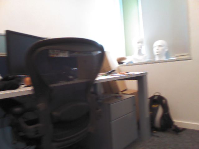
2.3. Pose Refinement using the 3D Model
Input
Frame
The output of a predictor such as (3) can be refined using
the 3D model. We represent the 3D model M : R3 →
[−1, 1] of a scene as a truncated signed distance function
[7] evaluated at continuous-valued positions by tri-linearly
interpolating the samples stored at voxel centers. The surface Mul0-‐Output
Predictor
of the model is then given by the level set M(y)=0 where y
Predictor
1
:
θ1
Predictor
2
:
θ2
Predictor
2
:
θM
is a 3D position in scene space.
Forest
1
Forest
2
Forest
M
Let xi ∈ R3 , i ∈ [k] be a set of observed 3D coordinates
in camera space. Then, a pose estimate H may be refined by
searching for a nearby pose that best aligns the camera space .
.
.
RANSAC
RANSAC
RANSAC
observations with the surface represented by M. Since M is
a (signed) distance to the surface, the value of [M(H̄xi )]2
will be small when H̄ aligns the camera space observations
closely to the current model of the surface. Thus, we can
refine a camera pose by minimizing the following nonlinear Rendered
Views
.
.
.
least-squares problem after initializing H̄ with the estimate
X
Href = argmin [M(H̄xi )]2 . (4)
H̄ i
This minimization problem can be solved by optimizing
over the rotational and translational components of H̄ using
the Levenberg-Marquardt algorithm (this is similar to the Model
Selector
Final
Pose
method of [6]). In our experiments we will evaluate the
effect of refinement on the poses estimated with the models Figure 1. Overview of the proposed method. We propose a two-
we compare. stage approach where the first stage generates M marginally rele-
vant predictions; and the second stage infers an accurate pose from
3. Proposed Approach the first stage’s predictions.
The direct regression approach is not rich enough to
Algorithm 1 Learn Multi-Output Predictor
model the one-to-many nature of the mapping between im-
ages and camera viewpoints. Our method for camera relo- 1: Inputs: S = {(Ij , Hj ) : j ∈ [n]}, M , ξ, `, σ
calization works by generating multiple hypotheses for the 2: Initialize with uniform weights: w0 ← n1 · 1
camera pose using a set (or ‘portfolio’) of regression-based 3: Θ0 ← {}
predictors and then selecting the best hypothesis using the 4: for t = 1, . . . , M do
reconstruction error. In some sense, this can be seen as a 5: Θt ← Θt−1 ∪ TrainForest[19] (S, wt−1 )
regression-based approach for solving the inverse problem 6: wt ← UpdateWeights(Θt , wt−1 , `, ξ, σ) (see (7))
defined in (1). More formally, given multiple predictors 7: end for
{g(·; θ m ) : θ m ∈ Θ} and a choice ξ of reconstruction error, 8: return ΘM
we approximate (1) by
3.1. Learning Marginally-Relevant Predictors
f (I; Θ, ξ) = argmin ∆ξ (I, R(g(I; θ m ); M)) . (5)
g(I;θ m ) An approach to learning a diverse set of predictors is to
Thus, the inversion amounts to computing the errors corre- train each of the predictors on different data, e.g., [9, 12].
sponding to each predictor output and taking the minimum. The key question here is to decide which data to use for train-
Fig. 1 presents an overview of the architecture we propose. ing each predictor. Equivalently, the problem can be posed
For this approach to succeed, we need to develop a learn- as the creation of multiple groups of training instances, such
ing algorithm for a set of predictors whose predictions are that training a predictor on each group yields an accurate set
marginally relevant, i.e., the predictions must cover the space of predictors. Note that groups may overlap or, more gener-
of all Hs well. In Section 3.1 we develop an algorithm for ally, assignments of instances to groups may be probabilistic.
training such a set of predictors, where each of them is of Further, the number of groups could be determined during
discriminative form as in (3). We then discuss in Section 3.2 the optimization.
how different choices for the reconstruction error affect the Grouping (or clustering) of data instances can be random
accuracy of our method. (e.g., [19]); performed in input space via algorithms such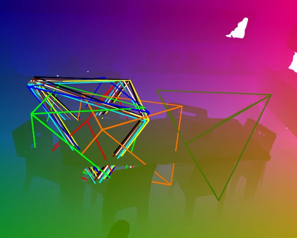
as k-means (e.g., [11]); or, better, driven by a task-loss [12].
Here, we pursue a new iterative loss-driven approach that
resembles boosting.
   Algorithm 1 summarizes our procedure for training a
multi-output predictor. At every iteration, a predictor of the
form (3) is trained using the learning algorithm in [19], with
the important difference that examples from each image j
contribute to the forest training objective in proportion to
some weight w(j). The first iteration uses uniform weights,
but weights on later iterations are a function of the loss
achieved by the predictors already trained. Importantly, this
mechanism allows multiple modes in the empirical distribu-
                                                                   Figure 2. Difficult case for the L1 reconstruction error due to model
tion of the training data to become re-weighted (as driven by
                                                                   distortion. Input depth (red channel) and depth raycast from ground-
the task-loss).                                                    truth (green channel) are shown superimposed. Observe how it
   The standard task-loss ` for camera pose estimation (de-        would be impossible to align the legs of both desks simultaneously.
fined in (2)) compares a single prediction with ground-truth.
To quantify the performance of a multi-output predictor Θt ,           We found the L1 distance to be sensitive to noise in the
we define the multi-output loss as                                 input depth images, and to distortions in the model (e.g., due
                                                                   to camera-tracking drift during model reconstruction). For
              `j (Θt ; ξ) = `(Hj , f (I; Θt , ξ)) ,         (6)    instance, see Fig. 2 where model distortion has led to a large
                                                                   distance between the input and the depth rendered from the
where f (I; Θt , ξ) is simply the camera pose hypothesis           ground-truth camera pose.
corresponding to the lowest reconstruction error among the             One way to make the distance robust to model-mismatch
outputs of predictors trained in iterations [t] – as defined       is to concentrate on shape. For instance, this can be done
in (5). Equipped with a multi-output loss we define the            through the use of a symmetric chamfer distance on edges de-
following weight update rule                                       tected on the depth frames (2DDT). This approach, however,
                                                               is problematic in that edge detection is also very sensitive to
             wt−1 (j)                −`j (Θt ; ξ)
    wt (j) ←               1 − exp                   , (7)         input noise and in that it completely ignores valuable depth
                 Zt                      σ2                        information.
                                                                       A robust error that we found superior to L1 is close to the
where Zt is a normalization factor and parameter σ roughly
                                                                   error used in the objective (4) of our model-based refinement
controls the diversity of the predictors – higher σ allowing
                                                                   algorithm
larger weight ranges. This update rule adjusts the weight of
individual training instances based on the loss incurred by
                                                                                                        X
                                                                            ∆3DDT (I, R(H; M)) =            | M(Hxi ) | .      (9)
the multi-output model.                                                                                     i
    It is important that during training we use the same defi-
                                                                   We refer to this reconstruction error as 3D-Distance Trans-
nition of multi-output loss as will be used at test-time. This
                                                                   form (3DDT). An additional benefit of 3DDT compared to
means we should use the same task-loss ` in (6) and the
                                                                   L1 or 2DDT is that it does not require raycasting.
same reconstruction error ξ in (5), (6) for both training and
testing.                                                           4. Hypothesis Aggregation
3.2. Selecting a Good Hypothesis                                      The performance of the reconstruction errors above is
   Here we study the problem of selecting a good camera            impaired by noise in the input data and problems in the 3D
pose estimate from a set of candidates {Hm : m ∈ [M ]}.            models such as missing data or distortion. This led us to
More specifically, we investigate the effectiveness of several     pursue the aggregation of poses in a way reminiscent of
reconstruction errors, which we denote by ξ in (5).                other ensemble methods. Algorithm 2 summarizes our pose
   Let Din denote the input depth image and DH denote a            aggregation procedure. It takes as arguments a set of pose
depth image raycast using pose estimate H and 3D model             hypotheses {Hm : m ∈ [M ]}; parameters δ and  for the
M. As a first choice for ξ consider the L1 distance                clustering of hypotheses; and parameters ξ and ζ for cluster
                                                                   scoring and selection.
      ∆L1 (I, R(H; M)) =
                              X
                                  | Din (i) − DH (i) | , (8)          Procedure ‘Cluster’ performs agglomerative clustering
                                 i
                                                                   on the poses using distance measure δ(H, H 0 ). Clustering
                                                                   stops when the distance between clusters exceeds . We ex-
where the summation is over pixels.                                plored several options for distance δ(H, H 0 ) between poses
2.3. Both the RGB and depth components of the input frames
exhibit ambiguities (e.g., repeated steps in Stairs), speculari-
ties (e.g., reflective cupboards in RedKitchen), motion-blur,
differing lighting conditions, flat surfaces, and sensor noise.
Metrics. Following previous work, we report accuracy as
the percentage of test frames for which the inferred camera
pose passes a correctness criterion. A correct pose must
be within a 5cm translational error and 5◦ angular error of
ground-truth (for comparison, the scenes have sizes up to
(a) Predictions. (b) Cluster means. (c) Best cluster. 6m on a side). This metric corresponds to the 0/1 loss,
Figure 3. Ambiguities on scene Stairs and results from our two-
stage approach. (a) M predictions shown as camera frusta; ground- 0 if δt (Hj , H) < t
truth (white); and selector’s pick (black). (b) Clusters (means) and δr (Hj , H) < r ,
PCj (H; t, r) = (12)
created during aggregation. (c) Poses in best-scoring cluster (pink);
1 otherwise
cluster mean (magenta); and ground-truth (white).
Algorithm 2 Aggregation of Pose Hypotheses where δt and δr are translational and rotational pairwise dis-
tances respectively; t = 5cm; and r = 5◦ .
1: Input: H = {Hm : m ∈ [M ]}, δ, , ξ, ζ
We report model performance at every iteration of train-
2: C ← Cluster(H, δ, ) see Section 4
ing, i.e., accuracy of the pose minimizing (5) (the selector’s
3: C ← argminC∈C Score(C, ξ, ζ) see (11)
pick) for sets of predictors [t] for t ∈ [M ]. For intermedi-
4: return Mean(C)
ate models, i.e., t < M , no aggregation is used since the
aggregation procedure was tuned on validation data for full-
including: Euclidean distance between the translation com- models only (i.e., using all M predictors). Thus, we only
ponents, angular distance between the rotation components, report accuracy for aggregate poses given M predictions.
and absolute difference on reconstruction errors, i.e., We report an ‘Oracle’ metric which is an upper-bound
on the performance of the selector. The Oracle metric is
| ∆ξ̄ (I, R(H; M)) − ∆ξ̄ (I, R(H 0 ; M)) |. (10)
the obtainable accuracy if we could always chose the best
Once the poses are clustered we use the following rule to prediction within the set of candidates. As before, we report
score clusters Oracle performance for models at every iteration.
Baselines. We compare our approach against the model
ζ |C|−1 X of [19] that was shown to achieve state-of-the-art camera
Score(C) ← ∆ξ (I, R(H; M)) . (11)
|C| relocalization on RGB-D data. To obtain an even stronger
H∈C
baseline, we extended the RANSAC optimization of [19]
This is a voting mechanism with a preference for larger to output the M best hypotheses (‘M -Best’). We refer to
clusters whenever ζ < 1. Finally, we take the ‘mean’ of the the first baseline as CVPR13 and to the latter as CVPR13 +
poses in the best-scoring cluster as our aggregate prediction. M -Best. Note that the CVPR13 baseline is equivalent to the
More precisely, we combine the poses in the cluster linearly predictor trained (with uniform weights) at the first iteration
with uniform weighting as suggested in [2]. of Algorithm 1 (t=1 in the plots).
Parameters for clustering and scoring, as summarized in For the CVPR13 + M -Best baseline we report perfor-
Algorithm 2, were tuned on held out validation data. mance on the first t-Best hypotheses for t ∈ [M ]. Also, we
tune the aggregation procedure and report aggregate pose
5. Evaluation accuracies using all M hypotheses.
Train and test samples. For each scene we took 1000 uni-
5.1. Experimental setup formly spaced frames from the (concatenated) training cam-
Dataset. We use the 7 Scenes dataset of [19] to evaluate era tracks. This was done to reduce training time and because
our approach. The dataset consists of 7 scenes (‘Chess’, contiguous frames are largely redundant.
‘Fire’, ‘Heads’, ‘Office’, ‘Pumpkin’, ‘RedKitchen’, and We also randomly sampled 1000 frames from the test
‘Stairs’) which were recorded with a Kinect RGB-D camera camera tracks of each scene. Half of these were used for tun-
at 640×480 resolution. Each scene is composed of several ing the parameters of the aggregation procedure (Algorithm
camera tracks that contain RGB-D frames together with 2) and the other half were used for testing. Note that for
ground-truth camera poses. The authors of the dataset used some scenes, e.g., Heads, this sampling yields all the avail-
the KinectFusion system [16] to obtain ground-truth poses able training and test data, while for others, e.g., RedKitchen,
and to reconstruct 3D models like those described in Section only a small fraction of the available data is used.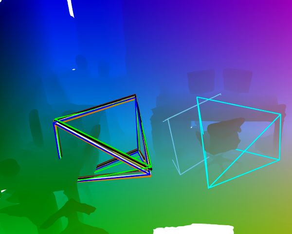
(a) Office.                                 (b) Pumpkin.                               (c) RedKitchen.
Figure 4. Qualitative results. Top row: input RGB-D frames. Bottom row: Pair-left: M predictions (colors); ground-truth (white); and
selector’s pick (black). Pair-right: Poses in best-scoring cluster (pink); cluster mean (magenta); and ground-truth (white).

5.2. Results                                                        our two-stage approach with the baselines. We report av-
                                                                    erage results over 5 runs for each scene (with different
Qualitative. Fig. 3 and 4 show illustrative prediction exam-
                                                                    random seeds) and over the 7 scenes. We trained mod-
ples. We observe that the predictions of the multi-output
                                                                    els using Algorithm 1 with parameters: M =10; ξ=3DDT;
model are indeed complementary and often cover multiple
                                                                    ` ∈ {PC, PCS}; and σ ∈ {0.01, 0.1, 0.2, 1.0}.
possibilities for ambiguous inputs. For example, multiple
steps in the Stairs scene (Fig. 3a), multiple desks/chairs in          Fig. 5b (top) shows average Oracle performance of the
the Office scene (Fig. 4a), and multiple sections of the long       baselines and several multi-output models. Fig. 5c (top)
flat cabinet in the Pumpkin scene (Fig. 4c).                        shows, for the same set of models, the average performance
Selector evaluation. We performed a set of experiments              when using 3DDT for selection and when using the aggrega-
to compare the effectiveness of our different pose-selection        tion Algorithm 2 (squares at t=10). While scene-averaging
mechanisms. These experiments were carried on all scenes            does hide somewhat contrasting behaviors on the different
and average results over the 7 scenes are reported.                 scenes, a few observations are warranted. First, the CVPR13
    We trained models using Algorithm 1 with parame-                + M -Best baseline does produce good hypotheses as shown
ters: M =8; ξ ∈ {L1, 3DDT, Oracle}; ` ∈ {PC, PCS};                  by the high Oracle performance. However, these are not
and σ ∈ {0.01, 0.1, 0.2, 1.0}. Here, PCS is a convex upper-         tuned to the selector and thus, it becomes more difficult to
bound on the 0/1 loss                                               select good hypotheses at test-time.
                                                                     The multi-output models trained with the PCS upper-
                            δt (Hj , H) δr (Hj , H)                 bound give the best results, achieving a ∼5% average ac-
   PCSj (H; t, r) = max                ,              . (13)
                                 t           r                      curacy improvement w.r.t. the CVPR13 + M -Best baseline.
                                                                    Aggregation (carried only on full-models and shown by the
We found re-weighting with PCS to be superior to PC be-
                                                                    square markers at t=10) achieved ∼1.5% average accuracy
cause the latter leads to trivial weightings of zero-weight for
                                                                    improvement w.r.t. the 3DDT selector.
examples with no loss and uniform weights for the rest of
the examples.                                                          Scene-averaging also hides effects of parameter σ of the
   Fig. 5a (top) compares L1 and 3DDT selector perfor-              re-weighting rule (7) but results on individual scenes (avail-
mance (averaged over all scenes). On average, 3DDT is               able in the supplementary) reveal that different scenes have
superior to L1 (which in preliminary experiments we found           different diversity requirements.
to be superior to 2DDT). We report only results for mod-            End-to-end with refinement. Fig. 5b (bottom) and 5c (bot-
els trained using ξ=Oracle as these are most meaningful             tom) show results for the same models when model-based
for comparing the efficacy of different selectors (otherwise        refinement is applied at test-time (Section 2.3). Trends are
predictors are trained to compensate for the specific recon-        roughly similar. Again, the CVPR13 + M -Best baseline has
struction error used during training).                              a very high average Oracle performance (in fact the highest
   We also compared selectors when hypotheses are refined           of all models). Still, the multi-output models are best on
using the model-based refinement from Section 2.3 at test-          the actual end-to-end evaluation and achieve a ∼1% average
time. Fig. 5a (bottom) shows average performance for this           accuracy improvement.
experiment. Again, 3DDT is superior.                                   Note that refinement was not used during training and
   Given the superior performance and efficiency of 3DDT,           thus the multi-output models are tuned for a different test
our subsequent and more extensive end-to-end evaluation is          scenario (i.e., that without refinement). For refined poses
limited to 3DDT.                                                    aggregation has a limited effect but still achieves a ∼0.5%
End-to-end (no refinement). These experiments compare               average accuracy improvement w.r.t. the 3DDT selector.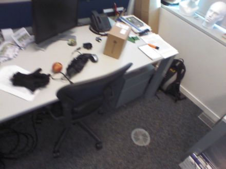
0.85
0.85
0.85
0.83
0.83
0.83
0.81
0.81
0.81
Average PC(5cm,5°)
0.79
0.79
0.79
0.77
0.77
0.77
0.75
0.75
CVPR13
+
M-‐Best
0.75
0.73
0.73
PCS-‐3DDT
1.0
0.73
PCS-‐3DDT
0.2
0.71
Oracle
0.71
PCS-‐3DDT
0.1
0.71
0.69
3DDT
0.69
PCS-‐3DDT
0.01
0.69
L1
PC-‐3DDT
1.0
0.67
0.67
0.67
1
2
3
4
5
6
7
8
1
2
3
4
5
6
7
8
9
10
1
2
3
4
5
6
7
8
9
10
0.85
0.92
0.92
0.83
0.91
0.91
0.81
0.90
0.90
Average PC(5cm,5°)
0.79
0.89
0.89
0.77
0.88
0.88
0.75
CVPR13
+
M-‐Best
0.87
PCS-‐3DDT
1.0
0.87
0.73
0.86
PCS-‐3DDT
0.2
0.86
0.71
Oracle
PCS-‐3DDT
0.1
0.69
3DDT
0.85
PCS-‐3DDT
0.01
0.85
L1
PC-‐3DDT
1.0
0.67
0.84
0.84
1
2
3
4
5
6
7
8
1
2
3
4
5
6
7
8
9
10
1
2
3
4
5
6
7
8
9
10
(a) Selector comparison (b) Oracle (c) 3DDT and aggregator (squares)
◦
Figure 5. Average PC(5cm, 5 ) (y-axis) over all scenes (5 runs per scene for b,c) vs. training iteration t (x-axis). Top row: no refinement.
Bottom row: refinement at test-time. (a) Performance of reconstruction errors when the predictors are fixed. (b,c) Comparison of multi-output
models and baselines. Legends indicate loss, selector and σ used during training. In (c) squares at t=10 correspond to aggregate poses.
Note that the CVPR13 baseline of [19] corresponds to the performance at t=1.
5.3. Computational Implications by running individual predictors on different cores.
As an aside, we note that greater performance gains could
We now contrast the gains achieved with our multi-output be attained by combining multi-output prediction and model-
prediction method with those obtained through model re- based refinement (i.e., refinement would need to be used
finement. In Fig. 6 we include average results for individual during training and testing of multi-output models).
scenes (5 runs per scene). Each plot compares the CVPR13 +
M -Best baseline combined with refinement at test-time, with
one multi-output model using no refinement. For each scene, 6. Conclusion
we selected one of the multi-output models from previous We have proposed a hybrid, discriminative-predictor
plots (i.e., we tuned σ) using the validation data. generative-selector, approach to inversion problems in com-
On these plots we see that our two-stage approach is su- puter vision that consists of: (i) a multi-output predictor; and
perior to the CVPR13 baseline (i.e., the model of [19]) on (ii) a ‘selector’ or ‘aggregator’ that is able to select or infer a
every scene. The accuracy improvements range from ∼5% good prediction given a set of predictions. We proposed a
on Pumpkin to ∼20% on Stairs. Further, on scenes Chess, procedure to train a set of predictors that make marginally
Office and RedKitchen our approach without refinement out- relevant predictions and showed that the training procedure
performs the CVPR13 + M -Best baseline with refinement. is able to tune the models for the selection stage to be used
However, on scenes Heads, Pumpkin and Fire, refinement at test-time. We demonstrated that the proposed approach
has a major effect with ∼44%, ∼14% and ∼12% accuracy leads to significant accuracy improvements when applied to
improvements, respectively. the problem of camera relocalization from RGB-D frames.
While both approaches, multi-output prediction and There are a number of interesting directions for future
model-based refinement, lead to significant improvements work. With regards to camera relocalization, while our ap-
they differ in their computational cost. The computational proach can cope with certain sources of failure (e.g., ambi-
complexity of our multiple-output prediction system at test- guity, multi-modality or test-train distribution mismatch), it
time scales linearly with the number of predictors. This would be beneficial to address other sources of failure for the
complexity could be significantly reduced by reusing tree model of [19]. Also, our approach is amenable to distributed
structures and only updating the leaf distributions when gen- learning, e.g., for camera relocalization in very large scenes.
erating multiple predictors. In contrast, the improvements For such cases, predictors could be learned on disjoints sub-
obtained through model-based refinement come at a high sets of training data (e.g., corresponding to different rooms)
computational cost because of the iterative nature. Further- and, like we do here, the selection mechanism would be
more, our multi-output method can be trivially parallelized responsible for determining the right prediction at test-time.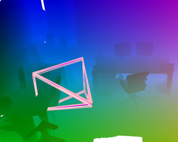
1.00
1.00
0.96
1.00
0.91
0.96
0.96
0.96
0.86
Average PC(5cm,5°)
0.92
0.92
0.81
0.92
0.88
0.88
0.76
0.88
0.71
0.84
0.84
0.84
CVPR13
+
M-‐Best
(refined)
0.66
0.80
0.80
0.61
0.80
PCS-‐3DDT
0.56
0.76
0.76
0.76
CVPR13
(refined)
0.51
0.72
0.72
0.46
0.72
CVPR13
0.68
0.68
0.41
0.68
1
2
3
4
5
6
7
8
9
10
1
2
3
4
5
6
7
8
9
10
1
2
3
4
5
6
7
8
9
10
1
2
3
4
5
6
7
8
9
10
(a) Chess (b) Fire (c) Heads (d) Office
1.00
1.00
0.80
1.00
0.96
0.96
0.75
0.96
Average PC(5cm,5°)
0.70
0.92
0.92
0.92
0.65
0.88
0.88
0.88
0.60
0.84
0.84
0.84
0.55
0.80
0.80
0.50
0.80
0.76
0.76
0.45
0.76
0.72
0.72
0.40
0.72
0.68
0.68
0.35
0.68
1
2
3
4
5
6
7
8
9
10
1
2
3
4
5
6
7
8
9
10
1
2
3
4
5
6
7
8
9
10
1
2
3
4
5
6
7
8
9
10
(e) Pumpkin (f) RedKitchen (g) Stairs (h) All scene average
Figure 6. Average PC(5cm, 5◦ ) (y-axis) (5 runs per scene) vs. training iteration t (x-axis). Comparison of the proposed approach without
refinement (orange) against the CVPR13 + M -Best baseline with model-based refinement (blue). For (a), (d) and (f) the accuracy
improvement from our approach is higher than that of model-based refinement. Further, on all scenes our approach is better than the CVPR13
baseline of [19] (performance at t=1). Squares at t=10 correspond to aggregate poses.
In the context of multi-output prediction it would be inter- [11] Q. Gu and J. Han. Clustered Support Vector Machines. In
esting to investigate the possibility of training models under AISTATS, 2013. 4
an explicit measure of diversity. For instance, we could de- [12] A. Guzman-Rivera, D. Batra, and P. Kohli. Multiple choice
vise a train-time loss that is augmented with a penalty for learning: Learning to produce multiple structured outputs. In
lack of diversity. Also interesting would be the evaluation of Proc. NIPS, 2012. 2, 3, 4
models such as determinantal point processes [14]. [13] G. Klein and D. Murray. Improving the agility of keyframe-
based SLAM. In ECCV, 2008. 1
References [14] A. Kulesza and B. Taskar. Determinantal point processes
for machine learning. Foundations and Trends in Machine
[1] S. Agarwal, N. Snavely, I. Simon, S. M. Seitz, and R. Szeliski. Learning, 5(2–3), 2012. 8
Building Rome in a day. In ICCV, 2009. 1 [15] V. Lepetit and P. Fua. Keypoint recognition using randomized
[2] M. Alexa. Linear combination of transformations. In SIG- trees. PAMI, 28(9), 2006. 1
GRAPH, 2002. 5 [16] R. Newcombe, S. Izadi, O. Hilliges, D. Molyneaux, D. Kim,
[3] S. Atiya and G. D. Hager. Real-time vision-based robot A. Davison, P. Kohli, J. Shotton, S. Hodges, and A. Fitzgibbon.
localization. Robotics and Automation, 1993. 1 KinectFusion: Real-time dense surface mapping and tracking.
[4] D. Batra, P. Yadollahpour, A. Guzman-Rivera, and In Proc. ISMAR, 2011. 1, 5
G. Shakhnarovich. Diverse m-best solutions in markov ran- [17] R. Salas-Moreno, R. Newcombe, H. Strasdat, P. Kelly, and
dom fields. In ECCV, 2012. 2 A. Davison. SLAM++: Simultaneous localisation and map-
[5] M. A. Brubaker, A. Geiger, and R. Urtasun. Lost! Leveraging ping at the level of objects. In CVPR, 2013. 1
the crowd for probabilistic visual self-localization. In CVPR, [18] S. Se, D. G. Lowe, and J. J. Little. Vision-based global
2013. 1 localization and mapping for mobile robots. Robotics, 2005.
[6] E. Bylow, J. Sturm, C. Kerl, F. Kahl, and D. Cremers. Real- 1
time camera tracking and 3D reconstruction using signed [19] J. Shotton, B. Glocker, C. Zach, S. Izadi, A. Criminisi, and
distance functions. In RSS, 2013. 3 A. Fitzgibbon. Scene coordinate regression forests for camera
[7] B. Curless and M. Levoy. A volumetric method for building relocalization in RGB-D images. In CVPR, 2013. 1, 2, 3, 4,
complex models from range images. In SIGGRAPH, 1996. 3 5, 7, 8
[8] A. Davison, I. Reid, N. Molton, and O. Stasse. MonoSLAM: [20] B. Williams, G. Klein, and I. Reid. Automatic relocalization
Real-time single camera SLAM. PAMI, 2007. 1 and loop closing for real-time monocular SLAM. PAMI,
[9] O. Dekel and O. Shamir. There’s a hole in my data space: 33(9):1699–1712, 2011. 1
Piecewise predictors for heterogeneous learning problems. In [21] Y. Yang and D. Ramanan. Articulated pose estimation with
AISTATS, 2012. 3 flexible mixtures-of-parts. In CVPR, 2011. 2
[10] G. N. DeSouza and A. C. Kak. Vision for mobile robot
navigation: a survey. PAMI, 24(2):237–267, 2002. 1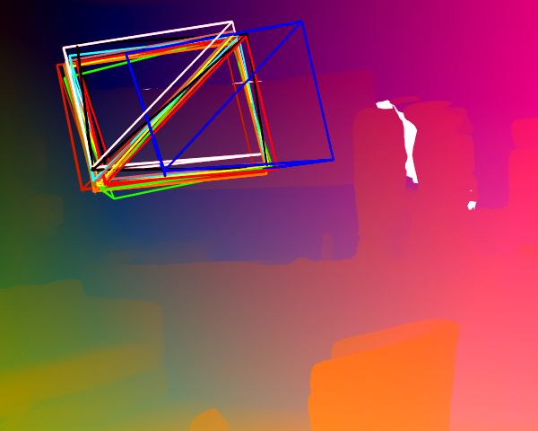

You can also read