ORStereo: Occlusion-Aware Recurrent Stereo Matching for 4K-Resolution Images
←
→
Page content transcription
If your browser does not render page correctly, please read the page content below
ORStereo: Occlusion-Aware Recurrent Stereo Matching for
                                                                     4K-Resolution Images
                                                              Yaoyu Hu1 , Wenshan Wang1 , Huai Yu1 , Weikun Zhen1 , Sebastian Scherer1

                                            Abstract— Stereo reconstruction models trained on small           binocular stereo datasets have an image size of fewer than
                                         images do not generalize well to high-resolution data. Training      2 million pixels (e.g. Scene Flow [5] 540 × 960 or a recent
                                         a model on high-resolution image size faces difficulties of data     one [6] with 1762×800) and a limited disparity range (e.g.
                                         availability and is often infeasible due to limited computing
                                         resources. In this work, we present the Occlusion-aware Re-          ∼200 pixels). They are far from what we face when using
arXiv:2103.07798v1 [cs.CV] 13 Mar 2021

                                         current binocular Stereo matching (ORStereo), which deals            real-world high-resolution images, e.g. 4K-resolution with a
                                         with these issues by only training on available low disparity        disparity range of over 1000 pixels. The next challenge is
                                         range stereo images. ORStereo generalizes to unseen high-            computing resources. Most deep-learning models consume
                                         resolution images with large disparity ranges by formulating         considerable amounts of GPU memory during training on a
                                         the task as residual updates and refinements of an initial
                                         prediction. ORStereo is trained on images with disparity ranges      small-sized image, e.g. the AANet [7] needs 2GB per sample
                                         limited to 256 pixels, yet it can operate 4K-resolution input        with a crop size of 288 × 756 and a disparity range of 192
                                         with over 1000 disparities using limited GPU memory. We              pixels. However, a higher resolution such as 4K resolution
                                         test the model’s capability on both synthetic and real-world         may require a crop width of over 2000 pixels to effectively
                                         high-resolution images. Experimental results demonstrate that        cover a disparity range of 1000 pixels. It is hard to train
                                         ORStereo achieves comparable performance on 4K-resolution
                                         images compared to state-of-the-art methods trained on large         a model with high-resolution data directly on typical GPUs
                                         disparity ranges. Compared to other methods that are only            since the memory consumption scales approximately in cubic
                                         trained on low-resolution images, our method is 70% more             with image dimension and disparity range.
                                         accurate on 4K-resolution images.                                       To this end, we choose to not rely on any high-resolution
                                                                                                              data. Our goal is trying to answer this question: how can a
                                                               I. I NTRODUCTION
                                                                                                              model that is trained on low-resolution data be general-
                                            High-resolution and accurate reconstruction of 3D scenes          ized to high-resolution images? Our philosophy is learning
                                         is critical in many applications. For example, LiDAR scan-           how to incrementally refine the disparity instead of predicting
                                         ners with a ∼5mm accuracy are typically used to build                it directly. Disparity refinement is less dependent on the size
                                         models for civil engineering analysis. However, this level of        of the input data. Also, it may be possible to trade time with
                                         accuracy is often not sufficient for detailed inspections and        accuracy by performing the refinement on a smaller scale but
                                         scanners are too expensive and heavy to be carried or flown          multiple times. We propose to handle high-resolution data
                                         by drones. Stereo cameras, on the other hand, are compact,           in a two-phase fashion. The first phase results in an initial
                                         and potentially high-resolution source of 3D maps if the             down-sampled disparity map. In the second phase, the same
                                         data can be effectively processed. Most of the recent high-          model recurrently refines the full-resolution disparity in a
                                         performance stereo matching models are learning-based,               patch-wise manner.
                                         however, a small number of them are focusing on high-                   While patch-wise processing is widely used for tasks
                                         resolution images.                                                   such as object detection, applying a similar strategy for
                                            Recent high-resolution oriented models need dedicated             stereo matching faces two issues. First, the small portion of
                                         training data to learn the ability to operate large disparity        occluded area gets enlarged in some patches, where occluded
                                         ranges or resort to a combination of models. Yang et al.[1]          regions cover most of those patches. These occlusion regions
                                         developed a deep-learning model (HSM) that can handle                do not have match in stereo images and disturb the refining
                                         a disparity range of 768 pixels. They collected a high-              process. ORStereo explicitly detects occlusions and stabilizes
                                         resolution (2056×2464) dataset to help the training. HSM             the recurrent updates. Second, the disparity range in the patch
                                         has impressive performance on the Middlebury dataset [2]             is still as large as it is in the original image, which is on
                                         which has a relatively larger image size than other public           one hand, out of the training distribution, and exceeded the
                                         benchmarks. For higher resolution such as 4K, Hu et al.[3]           patch size on the other. We find that by utilizing proper
                                         combined the SGBM [4] method with a deep-learning model              normalization techniques, a model can learn the ability to
                                         to deal with the high-resolution input.                              generalize to unseen disparity ranges.
                                            Data availability and limited computing resources are the            Our model is trained on publicly available datasets with
                                         main issues for training a high-resolution model. Typical            small image sizes. For high-resolution evaluations, we col-
                                                                                                              lected a set of 4K-resolution stereo images from both photo-
                                           1 Yaoyu Hu, Wenshan Wang, Huai Yu, Weikun Zhen, and
                                                                                                              realistic simulations and real-world cameras. The main con-
                                         Sebastian Scherer are with the Robotics Institute, Carnegie Mellon
                                         University.      {yaoyuh, wenshanw, huaiy, weikunz,                  tributions are summarized as follows.
                                         basti}@andrew.cmu.edu                                                   • We propose a two-phase strategy for high-resolution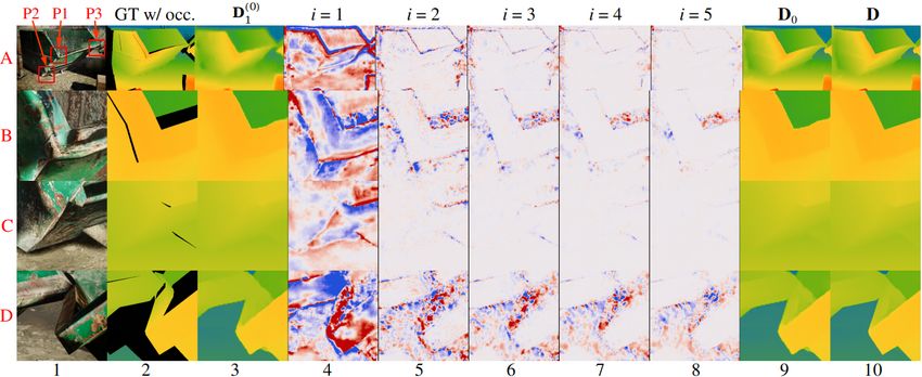
Fig. 1. ORStereo: Occlusion-aware Recurrent binocular Stereo matching. The whole model is trained with low-resolution data. During high-resolution
testing, ORStereo in used in two phases. The down-sampled disparity and occlusion are estimated in the first phase. These predictions are up-sampled and
patch-wise refined in the second phase.

       stereo matching using regional disparity refinements.                  occlusion issue in a small patch from a large image, our
   •   We design a novel structure to recurrently update the                  model recurrently handles the occlusion.
       disparity and occlusion predictions. The occlusions are                   Occlusion prediction Properly handling occlusion is im-
       explicitly predicted to guide the updates.                             portant for unsupervised learning models, e.g.[21], [22]. For
   •   We develop a new local refinement module equipped                      supervised models, Ilg et al.[23] demonstrated that a CNN
       with special normalization operations.                                 (convolutional neural network) can jointly estimate disparity
   •   We collect a set of 4K-resolution stereo images for                    and occlusion. We train ORStereo in a supervised manner.
       evaluation. This dataset is publicly available from the                To deal with large occluded areas in small patches, we chose
       project web page1 .                                                    to explicitly identify occlusions and let the model exploit this
                                                                              information. A recent work [24] shares a similar idea where
                          II. R ELATED WORK                                   occlusions are used to filter the extracted features before
                                                                              constructing the cost volume.
   Stereo matching is a widely studied topic and there are
                                                                                                       III. M ETHOD
many works both from geometry-based [8] and learning-
                                                                                 The ORStereo is trained on low-resolution images and
based research [9], [10], [11]. Many 3D perception tasks
                                                                              tested on 4K images (Fig. 1). It consists of 5 components
have a similar nature with binocular stereo reconstruction,
                                                                              (Fig. 2): a multi-level feature extractor (FE), a base disparity
such as multi-view stereo, monocular depth estimation, and
                                                                              estimator (BDE), a base occlusion mask estimator (BME), a
optical flow. We find many valuable inspirations and insights
                                                                              recurrent residual updater (RRU), and a normalized local re-
from all those tasks.
                                                                              finement component (NLR). When training on small images
   Residual prediction and recurrence As stated previously,
                                                                              (Fig. 1 Training, Fig. 2), BDE and BME learn to predict an
ORStereo learns to refine the disparity in a patch multiple
                                                                              initial disparity image and an occlusion mask, which are feed
times to obtain better accuracy. This process is similar to the
                                                                              into the RRU as initial values. The RRU works in a recurrent
residual prediction and recurrence. Many existing works train
                                                                              fashion gradually promotes prediction accuracy. At last, the
models to predict residuals to refine an initial prediction [12],
                                                                              NLR further refines the RRU’s prediction and outputs the
[13], [14], [15], [16]. However, these models update an
                                                                              final results. When testing on 4K image, we use the learned
initial prediction by a fixed number of steps or dimension
                                                                              model in a two-phase manner. In the first phase, our model
scales. In contrast, we introduce disparity improvements with
                                                                              estimates down-sampled disparity and occlusion mask. Then
variable steps in a recurrent way. Most of the recurrent
                                                                              in the second phase (Fig. 1 Testing), the RRU and NLR
models for 3D perception are designed for dealing with
                                                                              are reused to refine the enlarged patches in the original
sequential data, e.g. multi-view stereo models[17], [18]. As
                                                                              resolution. The key features of ORStereo is that the RRU
for binocular stereo, Jie et al.[19] utilized a recurrent neural
                                                                              and NLR are designed to be generalizable to large disparity
network (RNN) to keep track of the consistency between
                                                                              ranges. As a result, in testing time, when the 4K images with
the left and right predictions. Recently, RAFT applies an
                                                                              a large disparity range are presented, the RRU and NLR will
RNN to update optical flow prediction in a way similar to
                                                                              be able to improve the estimation accuracy even the disparity
an optimizer, thus the update converges as it proceeds [20].
                                                                              range is not seen in the training time.
Inspired by RAFT, we design a model to recurrently update
the disparity prediction without deterioration. To handle the                 A. Initial disparity and occlusion estimations
                                                                                 We place two dedicated components, namely the base
  1 https://theairlab.org/orstereo                                            disparity estimator (BDE) and the base occlusion mask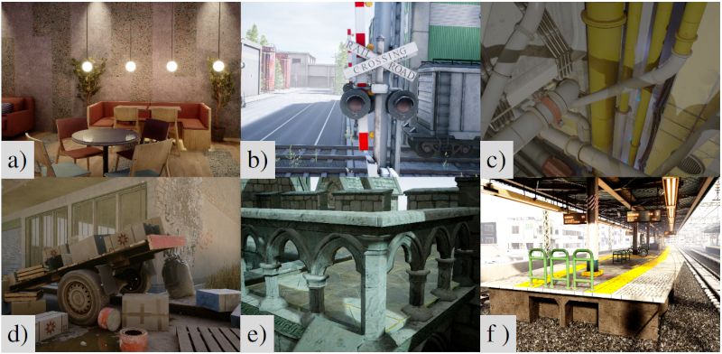
Fig. 2. Structure of ORStereo. We are using the same structure in both the first and second phases. F: feature tensor. D: disparity tensor. O: occlusion
mask. Ctx: context information. H: hidden state for the recurrent update. Superscripts: L (left), R (right), and W (warped). Subscripts: the level numbers.
BDE: base disparity estimator. BME: base occlusion mask estimator. RRU: recurrent residual updater. NLR: normalized local refinement.

estimator (BME), to calculate initial values for the RRU.                       ORStereo. Ideally, the warped image should roughly be the
The left and right images are first passed through a five-                      same compared with the left image in non-occluded regions.
level feature extractor, which has a simplified ResNet [25]                     Then patches from the left and the warped images should
structure. The extracted features are denoted as F in Fig. 2.                   now correspond to disparity values close to zero at non-
The BDE and BME take the F4 (Level 4) features at 1/16                          occluded pixels. Considering this phenomenon, we add a
of the input size. The BDE is implemented based on the                          pre-processing in the first phase to warp FR and assign an
3D cost volume technique similar to [1]. The BME predicts                       all-zero D1 to the RRU (Fig. 3). The RRU always has a zero
a initial occlusion mask for the RRU. It is designed as a                       D1 in the second phase.
encoder-decoder structure with skip connections. As shown                          The recurrent iterations. We design the RRU by aug-
in Fig. 2, let Di be the disparity tensor at Level i, we warp                   menting a GRU (gated recurrent unit) similar to [20]. The
FR                      W
  4 by D4 to get F4 . By comparing the feature pattern                          detailed model structure is illustrated in Fig. 4. The super-
            L        W
between F4 and F4 , the BME predicts the initial occlusion                      script (i) denotes the iteration step. For the ith iteration,
mask Oinit . In testing time, BDE and BME is only used in                                                 (i)           (i)
                                                                                the RRU computes RO and RD as the residuals for
the first phase. In the second-phase, the initial values for the                             (i)                   (i)
                                                                                occlusion O1 and disparity D1 based on the GRU’s hidden
RRU come from the results of the first phase.                                   variable H(i) . Similar to the [20], we keep a context feature,
                                                                                Ctx, as a constant reference to the initial state. The key
                                                                                differences from [20] are that ORStereo recurrently exploits
                                                                                the occlusion information to stabilize the recurrent iteration.
                                                                                   Since the RRU works in a recurrent way, during an
                                                                                evaluation after training, we can apply it like an optimizer by
                                                                                keeping it updating until a pre-defined criterion is satisfied.
                                                                                Here, unsupervised loss functions for similar perception tasks
                                                                                are reasonable criterion candidates. Later in the experiment
Fig. 3. The RRU pre-processing and iteration. Initial state (from top to        section, we tested the SSIM[27], which is widely accepted as
bottom): the hidden state H, context Ctx, multi-level features FL and
FR , disparity D1 , and occlusion O1 . O1 is obtained by resizing the O.
                                                                                a robust similarity measure for unsupervised methods. The
Blue dashed box: pre-processing in the first phase. Star: zero disparity. Red   RRU can keep updating a patch until the SSIM value between
dashed box: evaluation of the disparity and occlusion losses. The RRU           the original and warped images goes down. However, we
recurrently updates H, D1 , and O1 . The iteration stops when a fixed n is
reached or a convergence criterion triggers.
                                                                                found that the SSIM is not reliable and the RRU simply
                                                                                performs better with fixed and longer iterations.
B. Recurrent residual updater                                                      Residual update of occlusions. Iterations become un-
   To make the RRU work across two phases, we let the                           stable in occluded regions where little information is use-
RRU do a pre-process on the disparity and always begin                          ful for stereo matching. To improve robustness, the RRU
from zero disparity. Also, the RRU needs to properly handle                     explicitly handle the occlusion by the occlusion-augmented
                                                                                                              (i)
occlusions to stabilize the iteration. Note that the RRU takes                  H(i) (shown in Fig. 4). O1 is represented as a 2-channel
all the feature levels (FL and FR ) and updates disparity and                   tensor in ORStereo and supervised by cross-entropy loss,
                                                                                                                                     (i)
occlusion at Level 1 (D1 and O1 ) with 1/2 image width.                         which does not require a value-bounded O1 . However,
   Initial state with zero disparity. The RRU uses multiple                     this unbounded value cause problems for long recurrent
                                                                                                                 (i−1)
input types to start the iteration in both phases, as shown in                  updates. Fig. 4 shows that O1          first passes through a soft-
Fig. 3. In the training time, ORStereo only goes through                        max operator. This ensures an intermediate value-bounded
                                                                                                  (i)
the first phase. In the second phase as shown in Fig. 1,                        representation, SO , and keeps the gradients of the loss value
                                                                                        (i)
the full-resolution right image gets warped before going into                   w.r.t O1 from diminishing. Similar reasoning also explains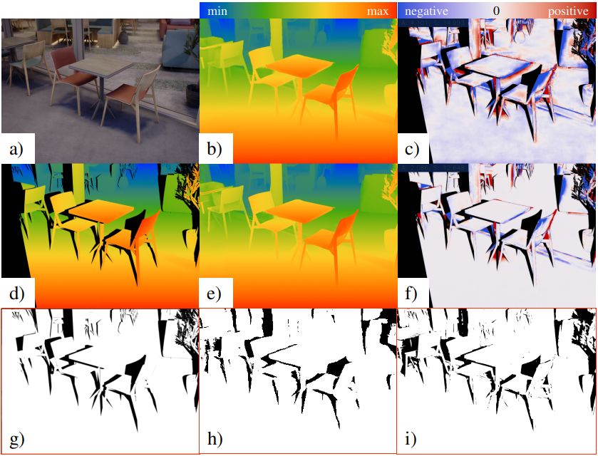
Fig. 4. The structure of the RRU. Residual update for D1 is element wise addition, (2). Residual update for O1 is defined in (1). The multi-level
cross-correlation is implemented by referencing [26].

the purpose of the Sigmoid operator, which bounds the value               where scalar m = mean(D0 ) and s = std(D0 ) are the mean
     (i)          (i)                            (i−1)
of RO . Here, RO is a single-channel tensor. O1        gets               and standard deviation of D0 . P normalizes the disparity,
updated by (1).                                                           and Q de-normalizes the residual value. Here, W serves as

              (i)

                             (i−1)

                                                (i)
                                                                          a local weight which encourages large residuals near local
         V O1 , j = V O1           , j − (−1)j RO       (1)               discontinuities.  is a constant hyperparameter. P and Q
                                                                          enable the NLR to generalize to large disparity ranges in
where function V (·, j) takes out the channel at index j from
                                                                          the second phase by making the NLR work in a normalized
a tensor and j ∈ {0, 1}. Equation (1) also makes the iteration
                                                                          disparity range.
more stable. Equation (2) gives the disparity update.
                        (i)
                      D1 = D1
                                 (i−1)
                                         + RD
                                             (i)
                                                                   (2)    D. Training losses
                                                                             We adopt a supervised scheme for all the outputs. The
C. Normalized local refinement                                            total training loss is defined as (5).
   Following the RRU, the normalized local refinement mod-
                                                                                    ltotal = λD             t     O          t

ule (NLR) adds a final update to the disparity D0 , as shown                                  4 SL D4 , D4 + λ CE O, O
                                                                                                 n
in Fig. 5. The NLR is designed to smooth the object interior                                    X
                                                                                                                    (i)

and sharpen boundaries by exploiting local consistency be-                                 + λD
                                                                                              1     (γ D )n−i+1 SL D1 , Dt1
                                                                                                  i=1
tween the disparity and the input image. The NLR extracts                                      n
its own features from the left image and works directly at                                                       (i)
                                                                                               X
                                                                                          + λO
                                                                                             1   (γ O )n−i+1 CE O1 , Ot1
the image resolution.                                                                             i=1
                                                                                          + λD SL D, Dt

                                                                                                                                             (5)
                                                                          where SL and CE are the smooth L1 and cross-entropy loss
                                                                          functions. n is the iteration number and from λD 4 to λ
                                                                                                                                  D
                                                                                                                                    are
                                                                          the constant weights for different loss values (see Table II).
Fig. 5. The normalized local refinement module (NLR). Refer to (3) to
(4) for definitions of some symbols.
                                                                          E. Working in the second phase
   The NLR also works in both phases. In the second phase                    We make patches out of four objects for the second phase:
the NLR faces a major challenge as disparity values go                    the left image, the warped right image, the disparity, and the
beyond the training range. The way the NLR handles this                   occlusion mask, all in the full-resolution. Our experiments
challenge is always working under a normalized disparity                  show that keeping small overlaps among patches achieves
range. In Fig. 5, the up-sampled disparity, D0 , is normal-               better results since accuracy may drop near the patch borders.
ized as D0 by function P . Then module G processes the                    In the overlap region, the disparity and occlusion predictions
feature FRe and D0 to produce residual RD . Then a de-                    are averaged across patches.
normalization function Q re-scales RD to RD . The final
                                                                                                  IV. E XPERIMENTS
disparity D is then obtained in the same way of (2). Module
G has an encoder-decoder structure. P and Q are defined                   A. Datasets and details of training
from (3) to (4).                                                            Our target is 4K-resolution stereo reconstruction with
              P (D0 ) = (D0 − m)/(s + ) = D0                      (3)    over 1000 pixels of disparity. ORStereo allows us to train
                                                                         with only small-sized images and a typical disparity range
             Q RD = (s + )RD = RD                                 (4)    around 200 pixels. We utilize several public datasets for the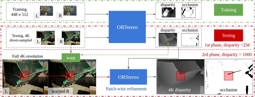
TABLE I
EPE METRICS OF ORS TEREO COMPARED WITH THE S OTA MODELS ON THE S CENE F LOW DATASET.
MCUA[28] Bi3D[29] GwcNet[30] FADNet[31] GA-Net[32] WaveletStereo[33] DeepPruner[34] SSPCV-Net[35] AANet[7] ORStereo (ours)
0.56∗ 0.73 0.77N 0.83 0.84 0.84 0.86 0.87 0.87∗ 0.74
ORStereo only goes through the first phase for this low-resolution test. ∗ Best values from individual works. N Finalpass. ORStereo is trained and tested on the cleanpass subset
of the Scene Flow dataset. Some samples are removed as suggested by the Scene Flow dataset.
training, i.e., the Middlebury dataset at 1/4 resolution [2], B. Evaluation the first phase on small images
the Scene Flow [5] dataset (∼35k stereo pairs), and the To evaluate the first phase of ORStereo on small-sized
TartanAir [36] datasets (∼18k pairs sampled). The Scene images, we train ORStereo on the Scene Flow dataset only
Flow and TartanAir datasets do not provide true occlusion and then compare it with the state-of-the-art (SotA) models.
labels. We generate them by comparing the left and right We limit the metric computation under 192 pixels, matching
true disparities. We will not use the KITTI dataset despite the SotA models. Table I lists the results on the testing
its popularity because it is hard to generate reliable dense set of the Scene Flow dataset measured in the average
occlusion labels from sparse true disparities. EPE (end point error) metric. ORStereo achieves comparable
Currently, no public stereo benchmark provides 4K- performance with the SotA models.
resolution data. So we collect a set of synthetic 4K-resolution
photo-realistic stereo images with ground truth disparity. C. Evaluation on high-resolution images
These images are captured by AirSim [37] in the Unreal For better performance and generalization ability across
Engine. We prepare 100 pairs of stereo images from 7 image sizes and disparity ranges, the Middlebury (at 1/4
simulated environments. Some cases may have a disparity resolution) and TartanAir datasets are added to the training.
range of over 1200 pixels. The evaluation cases in Fig. 7 We further augment the data with random color, random flip,
and 8 are from this dataset. Additional samples are shown and random scale similar to [1]. After training, we apply
in 6. The dataset is only used for evaluation and all images a 512×512 patch size with an overlap of 32 pixels in the
and ground truth disparities are available at the project page. second phase. In Sec. IV-D, after comparing the performance
with various iteration numbers, we make the RRU iterate for
10 steps in both the phases for the subsequent evaluations.
Although the training data have small size, we expect
ORStereo to learn the ability to refine a patch of disparity at
a higher resolution. We first show results on the Middlebury
dataset [2] with full resolution. This dataset is still considered
as hard for models trained on low-resolution data. We choose
three recent models (with available pre-trained weights)
that are trained with low-resolution data and have openly
evaluated their performance on the Middlebury dataset. Addi-
tionally, we include the HSM model[1], which can cover 768
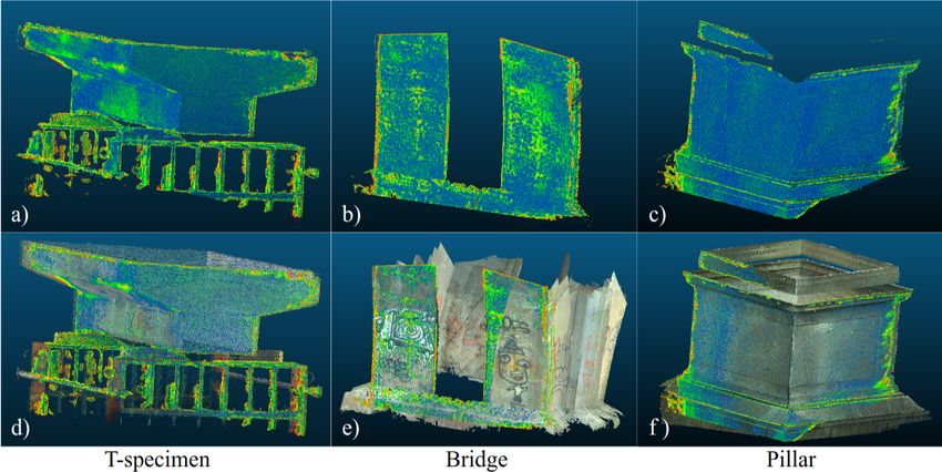
Fig. 6. Sample images from the 100 pairs of 4K-resolution stereo images. pixels of disparity after training on high-resolution images.
6 of 7 environments are shown: a) restaurant, b) factory district, c) under The quantitative results are listed in Table III. Trained on
ground work zone, d) city ruins, e) ancient buildings, f) train station.
smaller image size, we observed that ORStereo delivers
Training only happens in the first phase of ORStereo. We accuracy close to the SotA [1] trained on high-resolution
use a disparity range of 256 pixels and randomly crop the images. Later, when the resolution goes up to 4K, ORStereo
images to 448 × 512 pixels. We set the iteration number to can still maintain its performance.
4 for training the RRU. Similar works such as [20], [38]
TABLE III
also use fixed number of iterations during training. Other
C OMPARISON ON THE M IDDLEBURY EVALUATION DATASET
model constants are listed in Table II, where the loss weight
constants are chosen to balance the values from different loss Model AANet DeepPruner SGBMP ORStereo HSMN
& scale [7] 1/2 [34] 1/4 [3] full (ours) full [1] full
components. We train ORStereo with 4 NVIDIA V100 GPUs EPE 6.37 4.80 7.58 3.23 2.07
with a mini-batch of 24 for all experiments. Other training
NThis model is trained on high-resolution data. ORStereo achieves near
settings varying among different experiments will be shown SotA performance without training on high-resolution data. Non-occluded
separately. EPE is reported. All EPE values are associated with specific image scales.
All values are from the evaluation set and published on the website of
Middlebury dataset under the ”test dense avgerr nonocc” category.
TABLE II
T HE MODEL CONSTANTS OF ORS TEREO .
Some of the models in Table III are unable to operate
λD
4 λO λD
1 λO
1 λD γD γO
1e-6 32 2 2 1 2 0.8 0.8 4K-resolution images with a limited memory budget or their
effective disparity ranges are not enough, we down-sample
The values from λD 4 to λ
D are selected to make the loss components have
similar quantities in the end of a training.
the input until a model can handle it. Then the results are re-
scaled to the original resolution before evaluation. Besides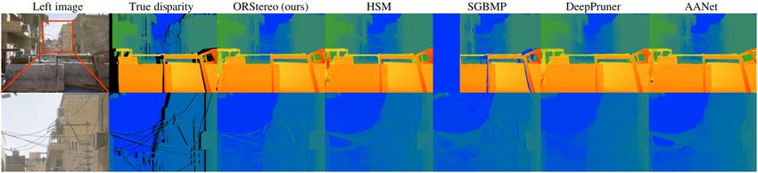
Fig. 7. Results on our 4K synthetic stereo images. The color map is the same as Fig. 8. Columns 3-7 are the disparity estimation of each model. Table IV
shows the quantitative statistics over all the 100 evaluation samples. Seeing thin structures is one of the motivation for high-resolution stereo reconstruction.
Our model exploits and reconstructs fine-grain details as shown in the zoom-in figures.

                                                                                                                 TABLE IV
the EPE metric. Evaluation is done with all the collected
                                                                                                 C OMPARISON ON THE SYNTHETIC 4K DATASET.
samples. Fig. 8 shows a sample output from ORStereo. In
                                                                                            Model                 Scale        Range     EPE     Mem (MB)
this figure, we can first compare the disparity predictions                                 AANet[7]              1/8          192       9.96    8366
from the two phases. The EPE of the first phase is 4.10 pixels                              DeepPruner[34]        1/8          192       8.31    4196
(Fig. 8 c, up-sampled back to 4K-resolution). ORStereo im-                                  SGBMP∗ [3]            1            256       4.21    3386
                                                                                            ORStereo (ours)       1            256       2.37    2059
proves this value to 2.09 pixels after the second phase (Fig. 8                             HSMN [1]              1/2          768       2.41    3405
f). As shown in Table IV, although ORStereo is trained
                                                                                  ORStereo shows the best results among the models trained on small
on small image size, its EPE is even lower than HSM on                            images. There are 100 pairs of stereo images. Scale: the down-sample scale
these 4K images with a smaller memory consumption. Fig. 7                         against the original image width. Range: the trained disparity range. EPE:
further provides us with a qualitative comparison. ORStereo                       non-occluded EPE. Mem: peak GPU memory (first/subsequent). ∗SGBMP
                                                                                  combines a learning-based and a non-learning-based model, only GPU
has the potential to fully utilize the fine-grained details in                    memory consumption is reported. NThis model is trained on high-resolution
high-resolution images and reconstructs thin structures that                      data.
are better captured by high-resolution images. ORStereo
achieves this at a cost of execution time because it needs
                                                                                  another one with less training data (remove all samples from
to refine multiple patches and the RRU iterates several steps
                                                                                  TartanAir). Furthermore, we test various iteration numbers
for each patch. On average, ORStereo spends about 15s for
                                                                                  and disable the RRU or NLR. All the above model variants
a single 4K-resolution image.
                                                                                  are evaluated on the same 100 pairs of 4K stereo images
                                                                                  used in Table IV. The results are shown in Table V. We
                                                                                  first observe that simply making the RRU iterate longer than
                                                                                  the training setting (4 steps) improves the overall accuracy.
                                                                                  Thus the RRU learns to work like an optimizer, which
                                                                                  gradually improve an initial prediction. However, this does
                                                                                  not hold with extensively long iterations, e.g. model F20 . The
                                                                                  FS model shows that monitoring the RRU by the SSIM is
                                                                                  not reliable. This may be due to the fact that SSIM fails
                                                                                  to distinguish stereo matching in texture-less and repeated
                                                                                  texture regions. The model variants (V1 -V4 ) regarding to less
                                                                                  training data and incomplete model structures all experience
                                                                                  a performance drop, meaning that ORStereo does benefit
                                                                                  from its special design. Notably, the V1 model that is trained
                                                                                  with less amount of data than the SotA methods in Table IV
                                                                                  still achieves the best EPE among the models trained on
Fig. 8. A 4K sample and ORStereo results. a) 4K Left image. b, c) disparity       low-resolution data.
and error of the first phase. d) ground truth disparity with occlusion. e,
f) disparity and error of the second phase. g) true occlusion mask. h, i)                                              TABLE V
occlusion prediction of the first and second phases. c) and f) are masked by
                                                                                         P ERFORMANCE COMPARISON BASED ON VARIOUS FACTORS .
the true occlusion from g). The EPE values are 4.10 in c) and 2.09 in f),
meaning that the disparity map gets improved in the second phase.                     Model       F4     F10    F15     F20        FS    V1      V2      V3      V4
                                                                                      All data    X       X      X       X         X       -      X      X        X
                                                                                     Occlusion    X       X      X       X         X      X        -     X        X
D. Ablation studies                                                                  RRU Iter.     4      10     15      20      SSIM     10      10      -       10
                                                                                       NLR        X       X      X       X         X      X       X      X         -
   For a better understanding on how various factors affect                            EPE       2.43    2.37   2.45    2.56      2.55   3.34    2.70   11.46    3.34

the performance of ORStereo, we additionally train two                            F4-F10: Full model with various RRU iteration numbers. F4 is the training setting.
                                                                                  F10 is the model used in Table III and IV. FS utilzes the SSIM to monitor RRU
models: one that has no explicit occlusion treatments (with                       iterations. V1-V4: model variants. V1 is trained without the TartanAir dataset, making
all the occlusion update shown in Fig. 4 removed), and                            the training set have less samples than the other SotA models shown in Table IV.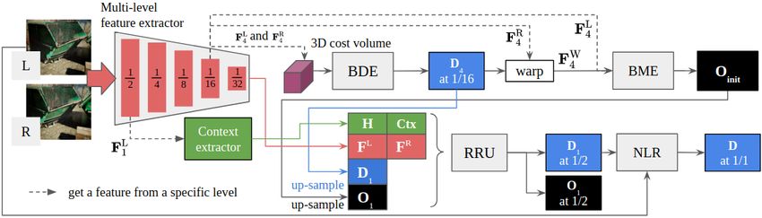
Fig. 9. The two phases of ORStereo. The color maps are the same as Fig. 8. Input: 4K-resolution. Row A: the first phase. 3 patches (512×512, P1-P3)
are cropped out for illustrating the second phase (Row B-D). Row B (P1): moderate disparity change and occlusion. Row C (P2): short disparity range,
limited occlusion. Row D (P3): large disparity jump, severe occlusion. Column 2, 3, 9, 10 are disparities. Column 4-8 show the first 5 updates made by
the RRU. The RRU quickly converges in the non-occluded regions after several iterations and oscillates in the occluded areas. The NLR (Column 10)
smooths and sharpens D0 (Column 9) in both phases. The results also indicate that the NLR can handle unseen disparities beyond the training range.

E. The characteristics of the two-phase procedure                            points num as a metric to measure the valid overlapped
   The RRU and NLR are the core components for ORStereo                      area. Both HSM[1] and ORStereo achieve similar millimeter-
to work across phases. To illustrate the characteristics of                  level precision. Notably, ORStereo obtains higher num than
the RRU and NLR, in Fig. 9, we show their behaviors in                       HSM, which means our model reconstructs more valid areas.
a complete first phase and 3 patches from the second phase.                  ORStereo is trained on small-sized synthetic data and utilizes
Fig. 9 shows that the RRU delivers stable and convergent                     fewer computation resources but still obtains competitive
updates in the non-occluded areas especially Row D in                        reconstruction results on real-world 4K stereo images.
the figure. In occluded regions, there is hardly any useful
information for stereo matching. However, inside a severely
occluded patch, ORStereo can use the detected occlusion to
guide the residual update, stabilizing the updates in the non-
occluded regions.

F. Evaluation on real-world 4K stereo images
   Evaluation on real-world high-resolution data is necessary
because ORStereo is trained with only synthetic images. We
set up a customized stereo camera with two 4K cameras
and a LiDAR and capture images around various objects.
To evaluate the stereo reconstruction results, we generate                   Fig. 10. Reconstruction results aligned with ground truth. Overlapping
dense point clouds as ground truth using a LiDAR-enhanced                    points are colorized by the point-to-plane distance to the ground truth by
                                                                             blue-green-yellow-red in an increasing manner. a)-c): points from ORStereo.
SfM [39] method. Using point clouds allows us to measure                     d)-f): the top row with the ground truth.
the metric error of the reconstructed model. For each scene,
all disparity maps from different viewpoints are converted                                            TABLE VI
to point clouds and are registered with the ground truth                       S TEREO RECONSTRUCTION RESULTS ON REAL - WORLD 4K IMAGES .
by the ICP method with an initial pose guess from the                                 Scene       T-specimen    Pillar   Bridge
SfM results. Both the ground truth and stereo reconstructed                           Frames           25        29        32
point clouds are down-sampled for efficiency. The results are                         Metrics     rmse num rmse num rmse num
shown in Fig. 10 and Table VI with three different scenes.                           HSM[1]        6.56 1.30 3.94 2.43 5.82 3.50
                                                                                     ORStereo      6.74 1.37 3.69 2.48 5.33 3.62
We use the mean point-to-plane distance (rmse) of all the
overlapping points between stereo point clouds and ground                    Frames: the total number of stereo pairs. rmse: point-to-plane
truth to measure the precision. A point is considered to                     distance in millimeters. num: valid overlapping points, unit 105 .
                                                                             rmse and num are averaged across all the frames of individual
have a valid overlap if it falls within 0.1m from any ground                 cases. Evaluations are conducted by down-sampling the point
truth point. Additionally, we use the number of overlapping                  clouds by a grid size of 5mm.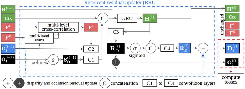
V. C ONCLUSIONS                                       [18] J. Liu and S. Ji, “A novel recurrent encoder-decoder structure for large-
                                                                                     scale multi-view stereo reconstruction from an open aerial dataset,” in
   We present ORStereo, a model that is trained only on                              CVPR, 2020.
small-sized images but can operate high-resolution stereo                       [19] Z. Jie, P. Wang, Y. Ling, B. Zhao, Y. Wei, J. Feng, and W. Liu, “Left-
images at inference time with limited GPU memory. In                                 right comparative recurrent model for stereo matching,” in CVPR,
                                                                                     2018, pp. 3838–3846.
testing time, ORStereo refines an initial prediction in a patch-                [20] Z. Teed and J. Deng, “Raft: Recurrent all-pairs field transforms for
wise manner at full resolution. By jointly predicting the                            optical flow,” arXiv preprint arXiv:2003.12039, 2020.
disparity and occlusion, the recurrent residual updater (RRU)                   [21] Y. Wang, Y. Yang, Z. Yang, L. Zhao, P. Wang, and W. Xu, “Occlusion
                                                                                     aware unsupervised learning of optical flow,” in CVPR, 2018.
can steadily update a disparity patch with severe occlusions.                   [22] A. Li and Z. Yuan, “Occlusion aware stereo matching via cooperative
With a special normalization and de-normalization sequence,                          unsupervised learning,” in Asian Conference on Computer Vision.
the normalized local refinement module (NLR) can gener-                              Springer, 2018, pp. 197–213.
                                                                                [23] E. Ilg, T. Saikia, M. Keuper, and T. Brox, “Occlusions, motion and
alize to unseen large disparity ranges. Our experiments on                           depth boundaries with a generic network for disparity, optical flow or
synthetic and real-world 4K-resolution images validate the                           scene flow estimation,” in ECCV, 2018.
effectiveness of ORStereo in both low- and high-resolution                      [24] S. Zhao, Y. Sheng, Y. Dong, E. I.-C. Chang, and Y. Xu, “Maskflownet:
                                                                                     Asymmetric feature matching with learnable occlusion mask,” in
stereo reconstruction. ORStereo achieves state-of-the-art per-                       CVPR, 2020.
formance without any high-resolution training data.                             [25] K. He, X. Zhang, S. Ren, and J. Sun, “Deep residual learning for image
                                                                                     recognition,” in Proceedings of the IEEE Conference on Computer
                     ACKNOWLEDGMENT                                                  Vision and Pattern Recognition (CVPR), June 2016.
                                                                                [26] D. Sun, X. Yang, M.-Y. Liu, and J. Kautz, “Pwc-net: Cnns for optical
   This work is supported by Shimizu Corporation. Special                            flow using pyramid, warping, and cost volume,” in CVPR, 2018.
thanks to Hayashi Daisuke regarding on-site experiments.                        [27] C. Godard, O. Mac Aodha, and G. J. Brostow, “Unsupervised monoc-
                                                                                     ular depth estimation with left-right consistency,” in CVPR, 2017.
                             R EFERENCES                                        [28] G.-Y. Nie, M.-M. Cheng, Y. Liu, Z. Liang, D.-P. Fan, Y. Liu, and
                                                                                     Y. Wang, “Multi-level context ultra-aggregation for stereo matching,”
 [1] G. Yang, J. Manela, M. Happold, and D. Ramanan, “Hierarchical deep              in CVPR, 2019.
     stereo matching on high-resolution images,” in CVPR, 2019.                 [29] A. Badki, A. Troccoli, K. Kim, J. Kautz, P. Sen, and O. Gallo, “Bi3d:
 [2] D. Scharstein, H. Hirschmüller, Y. Kitajima, G. Krathwohl, N. Nešić,         Stereo depth estimation via binary classifications,” in CVPR, 2020.
     X. Wang, and P. Westling, “High-resolution stereo datasets with            [30] X. Guo, K. Yang, W. Yang, X. Wang, and H. Li, “Group-wise
     subpixel-accurate ground truth,” in German conference on pattern                correlation stereo network,” in CVPR, 2019.
     recognition. Springer, 2014, pp. 31–42.                                    [31] Q. Wang, S. Shi, S. Zheng, K. Zhao, and X. Chu, “Fadnet: A fast and
 [3] Y. Hu, W. Zhen, and S. Scherer, “Deep-learning assisted high-                   accurate network for disparity estimation,” in ICRA. IEEE, 2020, pp.
     resolution binocular stereo depth reconstruction,” in ICRA. IEEE,               101–107.
     2020, pp. 8637–8643.                                                       [32] F. Zhang, V. Prisacariu, R. Yang, and P. H. Torr, “Ga-net: Guided
 [4] “Opencv stereosgbm class reference,” https://docs.opencv.org/                   aggregation net for end-to-end stereo matching,” in CVPR, 2019.
     4.5.0/d2/d85/classcv 1 1StereoSGBM.html, accessed: Nov. 16, 2020.          [33] M. Yang, F. Wu, and W. Li, “Waveletstereo: Learning wavelet coeffi-
 [5] N. Mayer, E. Ilg, P. Hausser, P. Fischer, D. Cremers, A. Dosovitskiy,           cients of disparity map in stereo matching,” in CVPR, 2020.
     and T. Brox, “A large dataset to train convolutional networks for          [34] S. Duggal, S. Wang, W.-C. Ma, R. Hu, and R. Urtasun, “Deeppruner:
     disparity, optical flow, and scene flow estimation,” in CVPR, 2016,             Learning efficient stereo matching via differentiable patchmatch,” in
     pp. 4040–4048.                                                                  ICCV, 2019.
 [6] G. Yang, X. Song, C. Huang, Z. Deng, J. Shi, and B. Zhou, “Driv-           [35] Z. Wu, X. Wu, X. Zhang, S. Wang, and L. Ju, “Semantic stereo
     ingstereo: A large-scale dataset for stereo matching in autonomous              matching with pyramid cost volumes,” in ICCV, 2019.
     driving scenarios,” in CVPR, 2019.                                         [36] W. Wang, D. Zhu, X. Wang, Y. Hu, Y. Qiu, C. Wang, Y. Hu, A. Kapoor,
 [7] H. Xu and J. Zhang, “Aanet: Adaptive aggregation network for                    and S. Scherer, “Tartanair: A dataset to push the limits of visual slam,”
     efficient stereo matching,” in CVPR, 2020.                                      arXiv preprint arXiv:2003.14338, 2020.
 [8] T. Taniai, Y. Matsushita, Y. Sato, and T. Naemura, “Continuous 3d          [37] S. Shah, D. Dey, C. Lovett, and A. Kapoor, “Airsim: High-fidelity
     label stereo matching using local expansion moves,” IEEE transactions           visual and physical simulation for autonomous vehicles,” in Field and
     on pattern analysis and machine intelligence, vol. 40, no. 11, pp.              Service Robotics, 2017.
     2725–2739, 2017.                                                           [38] Z. Bai, Z. Cui, J. A. Rahim, X. Liu, and P. Tan, “Deep facial non-rigid
 [9] A. Kendall, H. Martirosyan, S. Dasgupta, P. Henry, R. Kennedy,                  multi-view stereo,” in CVPR, 2020.
     A. Bachrach, and A. Bry, “End-to-end learning of geometry and              [39] W. Zhen, Y. Hu, H. Yu, and S. Scherer, “Lidar-enhanced structure-
     context for deep stereo regression,” in ICCV, Oct 2017.                         from-motion,” in ICRA. IEEE, 2020, pp. 6773–6779.
[10] J.-R. Chang and Y.-S. Chen, “Pyramid stereo matching network,” in
     CVPR, 2018, pp. 5410–5418.
[11] Y. Yao, Z. Luo, S. Li, T. Fang, and L. Quan, “Mvsnet: Depth inference
     for unstructured multi-view stereo,” in ECCV, 2018.
[12] J. Pang, W. Sun, J. S. Ren, C. Yang, and Q. Yan, “Cascade residual
     learning: A two-stage convolutional neural network for stereo match-
     ing,” in ICCV Workshops, 2017.
[13] X. Song, X. Zhao, H. Hu, and L. Fang, “Edgestereo: A context
     integrated residual pyramid network for stereo matching,” in ACCV.
     Springer, 2018, pp. 20–35.
[14] S. Khamis, S. Fanello, C. Rhemann, A. Kowdle, J. Valentin, and
     S. Izadi, “Stereonet: Guided hierarchical refinement for real-time edge-
     aware depth prediction,” in ECCV, 2018, pp. 573–590.
[15] R. Chen, S. Han, J. Xu, and H. Su, “Point-based multi-view stereo
     network,” in ICCV, 2019.
[16] P. L. Dovesi, M. Poggi, L. Andraghetti, M. Martı́, H. Kjellström,
     A. Pieropan, and S. Mattoccia, “Real-time semantic stereo matching,”
     in ICRA. IEEE, 2020, pp. 10 780–10 787.
[17] Y. Yao, Z. Luo, S. Li, T. Shen, T. Fang, and L. Quan, “Recurrent
     mvsnet for high-resolution multi-view stereo depth inference,” in
     CVPR, 2019.
You can also read