3D general-measure inversion of crosswell EM data using a direct solver

Journal of Geophysics and Engineering
Journal of Geophysics and Engineering (2021) 18, 124–133 doi:10.1093/jge/gxab001

3D general-measure inversion of crosswell EM data
using a direct solver
 1,*
Xuan Wang , Jinsong Shen1 and Zhigang Wang2
1
 Geophysical College, China University of Petroleum-Beijing, Beijing, 102249, China

 Downloaded from https://academic.oup.com/jge/article/18/1/124/6137303 by guest on 23 October 2021
2
 Bureau of Geophysical Prospecting INC., China National Petroleum Corporation, Zhuozhou, 072750, China
*
 Corresponding author: Xuan Wang. E-mail: waangxuuaan@163.com

Received 24 September 2020, revised 24 December 2020
Accepted for publication 5 January 2021

Abstract
We present a three-dimensional (3D) general-measure inversion scheme of crosswell
electromagnetic (EM) data in the frequency domain with a direct forward solver. In the forward
problem, we discretised the EM Helmholtz equation by the staggered-grid finite difference
(SGFD) scheme and solved it using the Intel MKL PARDISO direct solver. By applying a direct
solver, we simultaneously solved the multisource forward problems at a given frequency. In the
inversion, we integrated a general measure of data misfit and model constraints with linearised
least-squares inversion. We reconstructed a model with blocky features by selecting the
appropriate measure parameters and model constraints. We used the adjoint equation method to
explicitly calculate the Jacobian matrix, which facilitated the determination of an appropriate
initial value for the regularisation coefficient in the objective function. We illustrated the
inversion scheme using synthetic crosswell EM data with a general measure, the L2 norm, and,
specifically, two mixed norms.
Keywords: electromagnetic modelling, inverse problem, crosswell electromagnetic

1. Introduction Zhou (1989) carried out pioneering work on low-frequency
The three-dimensional (3D) electromagnetic (EM) inver- crosshole EM inversion by extending the acoustic inversion
sion problem has been a critical topic facing geophysicists technique to a complex wave number. On the basis of Zhou’s
over the past two decades. The impetus driving people’s work, Alumbaugh and Morrison developed an EM conduc-
research comes from the application of subsurface electri- tivity imaging technique using the second Born approxima-
cal conductivity distribution. In sedimentary formations, the tion to improve the accuracy of inverted conductivity im-
electrical conductivity mainly depends on the porosity, fluid ages (Alumbaugh & Morrison 1993). To calculate mod-
conductivity and saturation, and slightly depends on the els that contain large-scale anomalies, Newman (1995) ap-
formation temperature, permeability coefficient and pore plied the finite difference method to solve the differential-
geometry (Archie 1942; Keller 1988). Therefore, important equation (DE) formulation of Maxwell’s equations instead of
information, such as geological structure, fluid saturation, using the integral-equation (IE) approach. At the same time,
chemical composition and fracture direction, can be inferred the first field experiment was carried out at the Devine test
from the conductivity image. This knowledge can be applied site that is located southwest of San Antonio, Texas, USA
not only to reservoir characterisation, but also to mineral ex- (Wilt et al. 1995). The reconstructed resistivity from the
ploration, hydrogeology and chemical waste site evaluations. one-dimensional (1D) layered model inversion was consis-
 At the end of the 20th century, important progress was tent with the values from the induction log at the Devine
made in dealing with the crosswell EM inversion problem. test site. By separating and storing the data of different

124 © The Author(s) 2021. Published by Oxford University Press on behalf of the Sinopec Geophysical Research Institute. This is an Open Access article distributed under the terms of
 the Creative Commons Attribution License (http://creativecommons.org/licenses/by/4.0/), which permits unrestricted reuse, distribution, and reproduction in any medium,
 provided the original work is properly cited.

Journal of Geophysics and Engineering (2021) 18, 124–133 Wang et al.

calculation domains into hundreds of processors, Newman development of computing technology, however, the out-of-
& Alumbaugh (1997) took advantage of the message pass- core mode can store matrices on disk instead of in RAM
ing interface technique and the iterative solver of conjugate (Xiong et al. 2018), so that personal computers can also run a
gradients (CG) to perform a large-scale 3D EM inversion. large-scale EM inversion program with a sacrifice of time for
Using the regularisation method of linearised data and the data exchange.
modified Gram–Schmidt method, Shen et al. (2008) de- The main objective of this paper was to develop a
veloped a 2.5D crosshole EM inversion scheme with the general-measure inversion scheme for 3D crosswell EM data
forward responses calculated by the finite element method based on a direct solver. The scheme had three key com-
and the iterative solver of biconjugate gradient (Bi-CG). ponents: forward modelling, general measures and the in-
Based on an IE approach and Tikhonov regularisation, version algorithm. First, we used the staggered-grid finite
MacLennan et al. (2014) investigated the effects of com- difference (SGFD) method to discretise the DE formula-
plex conductivity on crosswell EM data. Colombo et al. tion of Maxwell’s equations and apply it to the Intel MKL
(2020) explored the use of the U-Net deep learning net- PARDISO direct solver to calculate large-scale sparse lin-
work for monitoring an EM-based reservoir. Zhang et al.

 Downloaded from https://academic.oup.com/jge/article/18/1/124/6137303 by guest on 23 October 2021
 ear system equations. Second, we presented one of the gen-
(2020) applied minimum support regularisation and the eral measures, the Ekblom norm, with its particular prop-
limited-memory Broyden–Fletcher–Goldfarb–Shanno (L- erty. Next, we showed how to solve the nonlinear inverse
BFGS) algorithm to solve the inverse problem and developed problem by linearised forward responses with the inversion
an ensemble-based history-matching framework to interpret scheme of the Ekblom norm and the minimum support (MS)
crosswell EM data. Fang et al. (2020) investigated a radial ba- constraint. Finally, we illustrated and discussed the general-
sis function neural network algorithm and compared it with measure inversion scheme through synthetic data of a
other five neural networks in a crosswell configuration. crosswell EM configuration.
 Almost all of these inversion schemes used L2 -norm as
their measure of data misfit and model structure. With
the help of structure constraints, however, their recon- 2. Forward modelling
structed images had a smooth and minimum structure, and We obtained model responses of crosswell configurations by
L2 -norm inversion could not recover images with blocky applying the approach of primary and secondary field de-
features. To solve this problem, researchers have published composition to the vector Helmholtz equations in the fre-
a number of articles about non-L2 norm inversion. Egbert quency domain. Assuming a time-harmonic dependence of
& Booker (1986) presented an iteratively reweighted least ej t and displacement currents are ignored, the equation for
square (IRLS) inversion for geomagnetic induction data with the secondary electric field Es in the frequency domain is
a hybrid measure of L1 -norm and L2 -norm. Farquharson written as follows:
& Oldenburg (1998) investigated general measures in the ( )
linear 1D magnetic data inversion and the nonlinear 1D ∇ × ∇ × Es + j Es = −j − p Ep , (1)
transient EM data inversion. Following the Ekblom norm
 where j2 = −1, denotes the angular frequency, represents
(Ekblom 1973), Zhang et al. (2000) applied 1D IRLS EM in-
 the magnetic permeability of free space, is the conductivity,
version to determine the bed boundary positions, which were
 p represents the background conductivity and Ep is the pri-
used as a priori information of two-dimensional (2D) inver-
 mary or background electric field. The total electric field E is
sion. By using the smoothness change information, Sun & Li
 given by
(2014) applied the dynamic Ekblom norm to different parts
of the model structure for automatic reconstruction of both E = Ep + Es . (2)
blocky and smooth models.
 Over the past decade, direct solvers have gradually be- Following Shen (2003), we computed the primary field
come popular tools for solving forward equations. There are Ep analytically, and we approximated the secondary field Es
two main reasons: (1) direct solvers only need to factorise with the SGFD discretisation method. We imposed Dirichlet
the system matrix once to solve solutions for multiple right- boundary conditions on the approximated calculation. This
hand sides (Newman 2013), which greatly reduces the time- resulted in a linear system of equations for a given frequency,
consuming multisource forward modelling; and (2) com- AEs = b, (3)
pared with iterative techniques, direct solvers are more sta-
ble and accurate, especially when dealing with models with where A is a Ne × Ne complex, sparse coefficient matrix,
low-frequency, nonuniform grids and large resistivity con- with Ne = 3Nx Ny Nz (where Ni is the number of cells in
trast (Gould et al. 2007; Grayver et al. 2013; Long et al. 2020). each direction). Ne -vector b is equal to the right-hand side
Although direct solvers have many advantages, their disad- of equation (1) that contains the source information of the
vantage is obvious: huge memory consumption. With the secondary field and boundary conditions.

 125

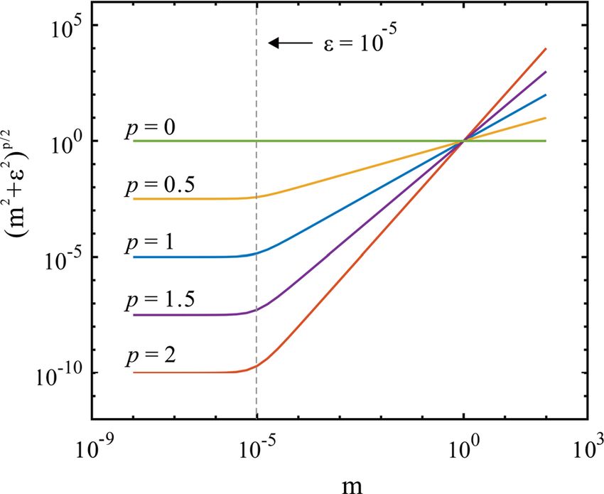
Journal of Geophysics and Engineering (2021) 18, 124–133 Wang et al.

 For the 3D crosswell EM problem, we had to solve the
multisource multifrequency forward equation (3) in the for-
ward modelling and sensitivity calculation. We used the In-
tel MKL PARDISO direct solver to simultaneously calculate
multisource large sparse linear equations at a given frequency
(Schenk & Gärtner 2002; Schenk & Gärtner 2004).
 Once we obtained the secondary electric field Es , we sub-
stituted it in equation (2) to yield the total electric field E.
We calculated the total magnetic field H from the total elec-
tric field E as follows:
 1
 H=− ∇ × E. (4)
 j 

 Downloaded from https://academic.oup.com/jge/article/18/1/124/6137303 by guest on 23 October 2021
3. General measures
 Figure 1. Ekblom norm with different p at = 10−5 .
Considering a Nm -vector m = (m1 , m2 , ..., mNm ) , a general
 T

measure of m is given by (Huber 1964)
 4. Inversion algorithm
 ∑
 Nm
 (m) = (mi ). (5) 4.1. Linearised inversion
 i=1 Considering that geophysical inversion is nonunique and the
 recovered model should be geologically interpretable, the ob-
When (m) = m2 or (m) = |m|, the measure becomes the
 jective function always consists of a data misfit function and
L2 or L1 norm. When (m) = |m|p , p ≥ 1, this measure be-
 model structure stabilising functions (Wang 2016):
comes the Lp norm of the vector. Thus, the weight on each
element of a vector m is controlled by parameter p. The larger g[ ( )]
 Φ (m) = Φd Wd dobs − f (m)
the parameter p, the more weight is imposed on large ele-
 [ ( )]
ments of a vector (Zhang et al. 2000). + Φgm Wc m + Wm m − mref , (7)
 Compared with the L1 norm, the L2 norm imposed more
weight on large mi during the process of minimisation. The g g
 where Φd and Φm are, respectively, symbols of the data mis-
image reconstructed from the L2 -norm inversion was rather fit function and model structure function defined by the
smooth as a result, and limited the occurrence of large ele- Ekblom norm. The complex Nd -vector d°bs is the observed
ments in the inverted model (Sun & Li 2014). For this reason, the data, f(m) is a forward response, mref denotes the refer-
we were able to recover features of sharp boundaries by ap- ence model, and Wd is a Nd × Nd weighting diagonal matrix
plying the L1 measure to the derivative of this model, and we that consists of the reciprocal of the data standard deviations.
smeared out features only when using L2 norm. In this paper, We used the Nm × Nm weighting matrices Wc and Wm for
we adopted a damped Lp norm proposed by Ekblom (1973): model constraint. The second term in equation (7) is also
 known as the stabiliser, which keeps the inversion stable and
 ( )p∕2
 (m) = m2 + 2 , (6) constrains the reconstructed model structure (Tikhonov &
 Arsenin 1977; Wang 2016). is the Lagrange multiplier,
where is a positive number. For brevity, it is referred to as and parameter determines the relative contributions of
the Ekblom norm. the smoothness term (i.e. Wc m) and the similarity term (i.e.
 Figure 1 shows the Ekblom norm with different p val- Wm (m – mref )) to the objective function (Oldenburg et al.
ues (i.e. 0, 0.5, 1, 1.5 and 2) at = 10−5 . If m ≫ , the 1993). We set = 0.1 (we discuss the selection of later).
Ekblom measure puts more weight on a large mi and less Once we defined the objective function, we could solve
weight on a small mi when the parameter p increased, which the inverse problem by minimising the nonlinear objective
led to a rather smooth image. As became larger, the mea- function with the linearised data. Assuming mk+1 is the
sure behaved like a sum-of-squares measure scaled by model perturbation of mk , the Taylor series of the forward
(Farquharson & Oldenburg 1998). Compared with the Lp responses f(m) at mk+1 without higher-order terms is given
norm, the Ekblom norm removed the singularity at m = 0 by the following:
when p = 1. We applied this general measure to perform ( ) ( )
crosswell EM inversion. f mk+1 = f mk + Jk Δmk , (8)

 126

Journal of Geophysics and Engineering (2021) 18, 124–133 Wang et al.

or package to calculate the updated model Δmk at the kth it-
 Δdk = JΔmk , (9) eration from the least-squares system (13). The gelsy rou-
 tine used the complete orthogonal decomposition of the sys-
where Jk is the Jacobian matrix at kth iteration and Δmk = tem matrix to calculate the solution of the linear least-squares
mk+1 − mk . Then, the objective function of Δmk is written problem (Anderson et al. 1999). Then, we obtain a new
as follows: model as follows:
 ( ) g[ ( )]
 Φ Δmk = Φd Wd Jk Δmk − Δdk mk+1 = mk + Δmk . (14)
 [ ( )
 + Φgm Wc mk + Δmk Until the misfit was less than the noise level or a given number
 ( )] of iterations had been reached, the inversion stopped. Other
 + Wm mk + Δmk − mref . (10)
 than the model constraint matrices discussed in the next sec-
The minimisation of the objective function (10), that is, tion, there are two matrices/parameters that we have not in-
 Φ( mk )∕ Δm = 0, yields the system of the normal equa- terpreted: the Jacobian matrix J and the Lagrange multiplier

 Downloaded from https://academic.oup.com/jge/article/18/1/124/6137303 by guest on 23 October 2021
tions, . We used the adjoint equation method to calculate the Jaco-
 [ kT T T ] bian matrix J (McGillivray et al. 1994) and, next, we discuss
 J Wd rd rd Wd Jk + WcT rcT rc Wc + WmT rmT rm Wm Δmk
 the selection of .
 = JkT WdT rdT rd Wd Δdk − WcT rcT rc Wc mk Based on the explicit calculation of the Jacobian matrix,
 ( ) we developed a new cooling strategy to select the Lagrange
 + WmT rmT rm Wm mref − mk , (11) multiplier . In the traditional cool strategy, the initial value
where rd , rc and rm are diagonal matrices (Sun & Li 2014): of was so large that the model constraints dominated data
 √ misfit (Oldenburg & Li 2005). More iterations needed to be
 [( ]p∕2−1 carried out until the value of decreased to a proper level.
 ( ))2
 rdii = p Wdi J Δmi − Δdi
 k k k
 + 2 , To solve this problem, we determined the initial value of 
 through the balance equation:
 (12a)
 g
 Φd ≈ Φgm . (15)
 √
 [( ]p∕2−1
 ( k ))2 For the least-squares system in equation (13) at p = 1, the
 rcii = p Wci mi + Δmi
 k
 + 2 , (12b) initial is given by the following:
 /
 √ ‖rW ‖
 √ ‖ ‖ ‖ c c‖
 [( ( ))2 ]p∕2−1 = ‖r d W d J k ‖ ‖ ‖ . (16)
 ‖ ‖∞ ‖rm Wm ‖
 rmii = k k ref
 p Wmi mi + Δmi − mi + 2 . ‖ ‖∞
 We took the infinite norm of the matrix because el-
 (12c)
 ements in the Jacobian matrix were arranged in rows.
 So, the Lagrange multiplier at kth iteration is shown as
 If we set p = 2, all three matrices would become identity
 follows:
matrices I. So, the system of the normal equations defined by √
the Ekblom norm included the one defined by the conven- √
 k = k , (17)
tional L2 norm as a special case. When p = 1 and < m, the n
reconstructed image obtained from equation (11) was sim- where is an empirical constant, n is a non-negative constant
ilar to the one from the L1 -norm inversion. Matrices rd , rc and k is the number of iterations.
and rm acted as weighting coefficients for each element of the
data-weighting matrix (Wd ) and the model constraints ma-
trices (Wc and Wm ). 4.2. Model constraints
 Equation (11) can be simplified to the linear least-squares For 3D inversion, the model smoothness matrix Wc is com-
system, as follows: posed of the following three spatial components (Li &
 ⎡ rd W d J k ⎤ ⎡ rd Wd Δdk ⎤ Oldenburg 1996):
 ⎢ √ ⎥ ⎢ √ ⎥
 ⎢ rc Wc ⎥ Δm = ⎢
 k
 − rc Wc m k
 ⎥, Wc = x Wcx + y Wcy + z Wcz , (18)
 ⎢√ ⎥ ⎢√ ( ref ) ⎥
 ⎣ rm Wm ⎦ ⎣ rm Wm m − mk ⎦ where ( x , y , z ) are weighting coefficients in three di-
 y
 (13) rections, (Wcx , Wc , Wcz ) are the first-order difference op-
which results in a more accurate solution (Sasaki 2001). We erators, for the model x = 1, … , Nx , y = 1, z = 1 and
used the gelsy routine of the Intel MKL LAPACK software the first-order forward difference coefficient matrices are as
 127

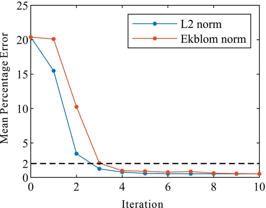
Journal of Geophysics and Engineering (2021) 18, 124–133 Wang et al.

Figure 2. Plan views at (a) y = 0 m, (b) x = 0 m and (c) z = 150 m. Circles denote transmitter wells and triangles denote receiver wells. White dotted
lines indicate the inverted area.

 Downloaded from https://academic.oup.com/jge/article/18/1/124/6137303 by guest on 23 October 2021
follows: We applied the MS constraint to the last term of the objec-
 tive function. The MS stabilising function was proposed by
 ⎛−1 1 ⋯ 0⎞ Last and Kubik to find the model with the smallest volume
 ⎜⋮ ⋱ ⋱ ⋮⎟ change compared with the reference model (Last & Kubik
 Wcx = ⎜ ⎟, 1983). Here, Wm is the diagonal matrix
 ⎜0 0 −1 1⎟
 ⎜ ⎟ 1
 ⎝0 0 ⋯ 0⎠ ⎛ √( )2 0 ⎞
 ⎜ m1 −mref1 + 2 ⎟
 ⎛−1 ⋯ ⋯ 0⎞ ⎜ ⎟
 0 0 1 0 Wm = ⎜ ⋱ ⎟,
 ⎜ ⋱ ⋮⎟⎟ ⎜ 1 ⎟
 ⎜ ⎜
 0 √( )2 ⎟
 ⎜ ⋱ ⋮⎟ ⎝
 ref
 mNm −mNm + ⎠ 2

 ⎜ ⎟ (20)
 ⎜ −1 0 ⋯ 0 1⎟
 Wc = ⎜
 y
 ⎟,
 ref
 where is the stability factor when (mi − mi ) → 0. Such a
 ⎜ 0 ⋯ ⋯ 0⎟
 diagonal weighting matrix has been used extensively in geo-
 ⎜ ⋱ ⋮⎟
 ⎜ ⎟ physics (Wang 1999). We applied an L-curve method that
 ⎜ ⋱ ⋮⎟ was similar to the optimisation of regularisation coefficients
 ⎜ ⎟ to find the optimal parameter (Portniaguine & Zhdanov
 ⎝0 0⎠
 1999).
 ⎛−1 0 ⋯ 0 1 0 ⋯ 0⎞
 ⎜ ⋱ ⋮⎟⎟
 5. Synthetic data example
 ⎜
 ⎜ ⋱ ⋮⎟ Next, we applied the inversion scheme to a 3D crosswell
 ⎜ ⎟ EM problem—that is, a synthetic crosswell EM survey over
 ⎜ −1 0 ⋯ 0 1⎟ an area of 400 × 400 × 400 m. Two 20 Ω ⋅ m-1 anomalous
 Wc = ⎜
 z
 ⎟.
 ⎜ 0 ⋯ ⋯ 0⎟ objects were embedded in a homogeneous half-space of 2
 ⎜ ⋱ ⋮⎟ Ω ⋅ m-1 (figure 2). A cuboid of size 120 × 40 × 40 m with
 ⎜ ⎟ its top at a depth of 140 m and another identical cuboid was
 ⎜ ⋱ ⋮⎟ placed 40 m below it. The two 200-m-deep source wells and
 ⎜ ⎟
 ⎝0 0⎠ two 200-m-deep receiver wells were placed around anoma-
 lies. We deployed 21 vertical magnetic dipole transmitters
 (19) at each well with 10 m intervals, and the receivers for each
 of the receiver wells had the same layout, which yielded
 For the case of y = 2, … , Ny , z = 2, … , Nz , 1764 source–receiver combinations. We inverted the vertical
 y
the coefficient matrices (Wcx , Wc , Wcz ) were consistent magnetic field component Ez of 370 Hz, which contained
with equation (19). The smoothness matrix of the full model 2% random noise.
Wc could be easily constructed using a triple-loop algo- The dotted rectangular area in figure 2 is the inverted area
rithm. This constraint is known as the flattest model (FM) used in the inversion algorithm, which was smaller than the
constraint. area used in the forward problem. For forward modelling, the
 128

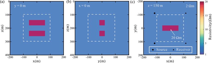
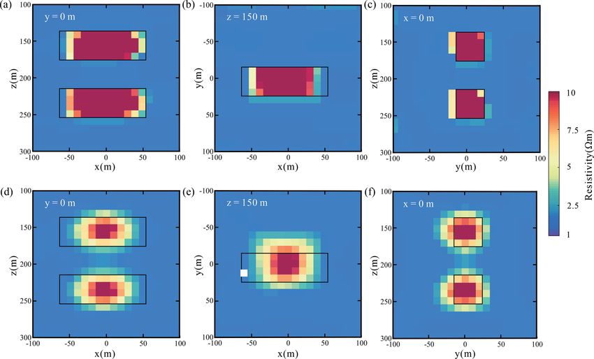
Journal of Geophysics and Engineering (2021) 18, 124–133 Wang et al.

 Downloaded from https://academic.oup.com/jge/article/18/1/124/6137303 by guest on 23 October 2021
Figure 3. Inversion results obtain by applying (a–c) Ekblom norm and (d–f) L2 norm.

model was discretised into the grid of 50 × 50 × 50 cells,
with a minimum cell size of 10 × 10 × 10 m and a
maximum size of 200 × 200 × 200 m, whereas the inverted
region contained 8000 (20 × 20 × 20) cells. It was critically
important to exclude receiver points from the inverted re-
gion in the inversion of the explicitly calculated Jacobian ma-
trix. When we used the adjoint equation method to explic-
itly calculate sensitivities, the receiver points had to be ex-
cluded from the inverted region. As a result, a number of sin-
gularities from the solution of adjoint equations were intro-
duced into Jacobian matrix, which made it difficult to solve
equation (13).
 The initial model for inversion was a homogeneous half-
space of 2 Ω ⋅ m-1 . We set the parameters of the Ekblom
norm as p = 1 and = 10−5 . We chose = 0.1, n = 2 and =
 Figure 4. Convergence plot for L2 norm (blue) and Ekblom norm (red).
5000 from our experiences. Several trial-and-error tests were
 The dashed line shows the noise level of 2%.
required to determine these values, especially beta. For these
model constraints, we set x = 1, y = 0.35, z = 0.35 and =
0.15. The misfit is calculated by the mean percentage error: smoothed out the boundaries of anomalies under the same
 model constraints. The reason for these results was that
 1 ∑ ||f (m)i − di ||
 Nd
 the Ekblom measure (p = 1 and = 10−5 ) put less weight
 misfit = × 100. (21)
 Nd i=1 |d | on large mi and more weight on small mi , which led to an
 | i|
 image with relatively sharp boundaries (Zhang et al. 2000;
Figure 3 shows the models obtained by the inversion with Sun & Li 2014). Although both inversions could correctly
the Ekblom norm and L2 norm. The Ekblom-norm inversion determine the position of the anomalies, they somewhat un-
achieved relatively blocky anomalies with the help of the derestimated the resistivity of the objects. Note that we set
FM and MS constraints, whereas the L2 norm inversion the upper limit of the resistivity in figure 3 to 10 Ω ⋅ m-1 , that
 129

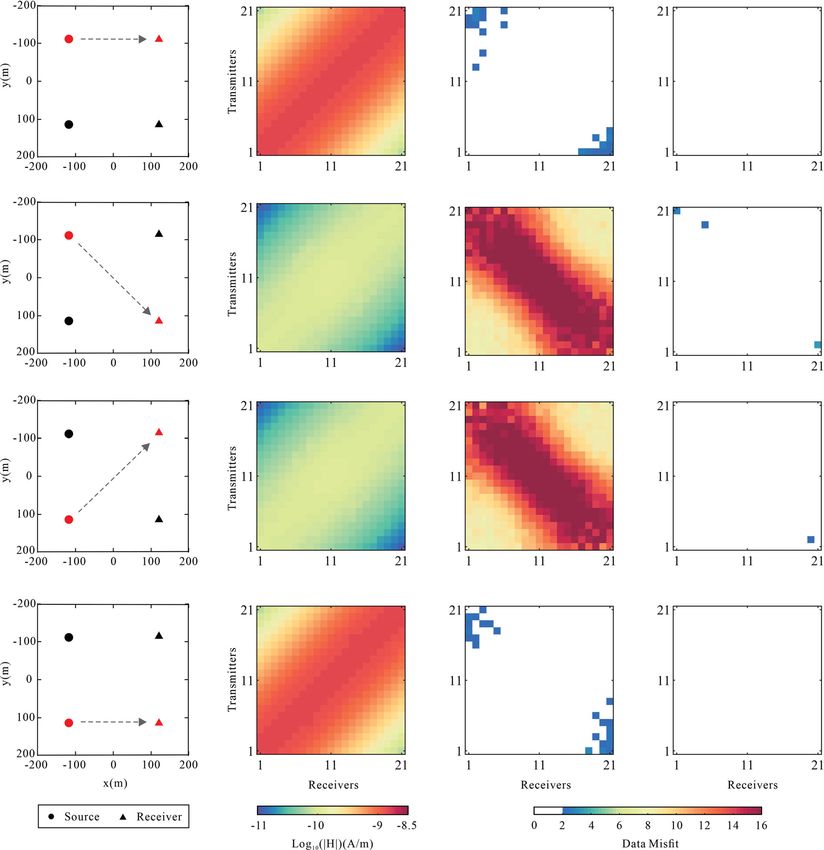
Journal of Geophysics and Engineering (2021) 18, 124–133 Wang et al.

 Downloaded from https://academic.oup.com/jge/article/18/1/124/6137303 by guest on 23 October 2021
Figure 5. Four source-receiver combinations (first column), amplitudes of the observed data (second column), mean percentage error of the predicted
data and the observed data before and after Ekblom-norm inversion, respectively (third and last column).

is, a half of the true model. The maximum resistivity value sures, however, we had to control the variable. To fully
of the anomalous bodies from the Ekblom-norm inversion illustrate the inversion results, we displayed amplitudes
was 13.2 Ω ⋅ m-1 , whereas that of the L2 -norm inversion was of the observed data for all observation systems and the
11.7 Ω ⋅ m-1 . data misfit for all source-receiver combinations before and
 Figure 4 shows the convergence rates of the inversions after the Ekblom-norm inversion shown in figure 5. The first
with two measures. Both inversions converged to a 2% column of figure 5 shows four observation systems, and the
data noise floor within ten iterations. The misfit of the second column shows the amplitudes of the observed data.
Ekblom-norm inversion at the first iteration showed few de- The third and last columns in figure 5 show data misfit at the
creases compared with the initial misfit, which suggested initial iteration and the sixth iteration. As shown in the last
that 5000 was not the optimal value of the Lagrange multi- column of figure 5, misfits of almost all source-receiver com-
plier . For the purpose of comparison between two mea- binations reached the noise level of 2%. Figure 6 shows the

 130

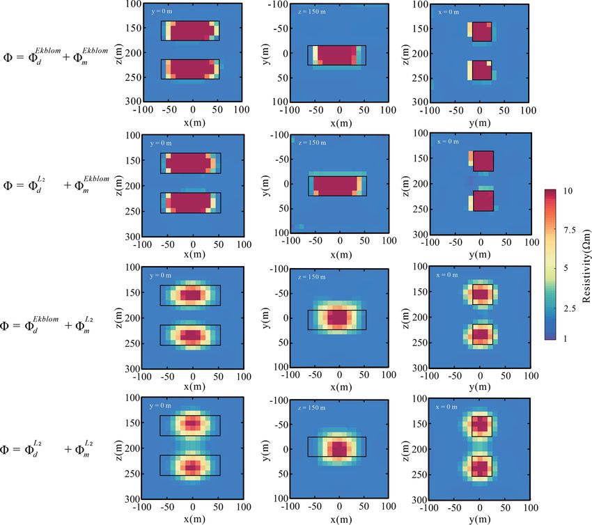
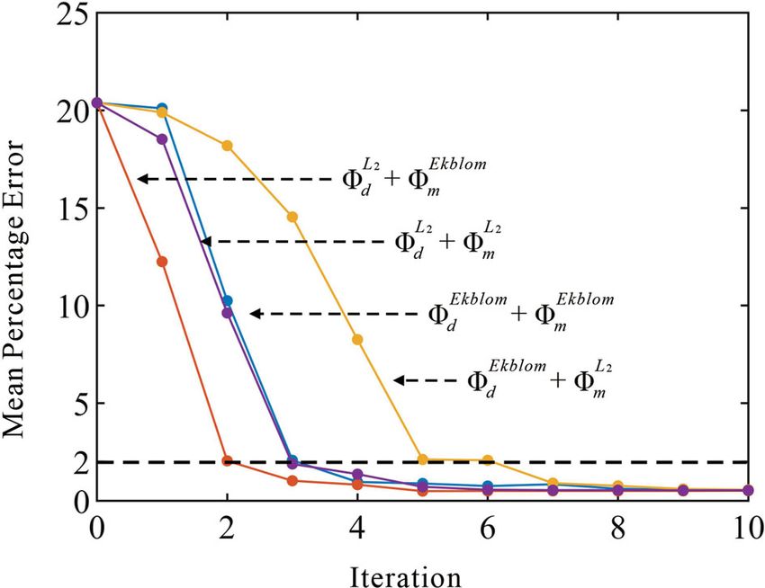
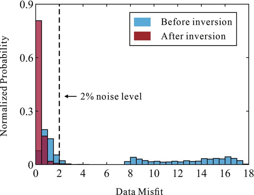
Journal of Geophysics and Engineering (2021) 18, 124–133 Wang et al.

 data misfit histogram before and after the inversion. After ten
 iterations, 99.3% of the predicted-data misfit of the Ekblom-
 norm inversion was less than the noise level of 2% and 96.7%
 of the misfit was less than 1%. The predicted-data graphs of
 the L2 norm were similar to figures 5 and 6, which are not
 shown because of the length of the paper.
 To investigate the influence of the data misfit term and
 model term with different measures on the inversion, we
 tested the inversion of two mixed norms. The objective func-
 tions of the two mixed-norm inversions were Φ = ΦEkblomd
 +
 L2 L2
 Φm and Φ = Φd + Φm , respectively. This was easy to
 Ekblom

 implement. For the former, we set p = 2 in rc and rm , whereas
 for the latter, we set p = 2 in rd . Figure 7 shows the inver-

 Downloaded from https://academic.oup.com/jge/article/18/1/124/6137303 by guest on 23 October 2021
 sion results of the two mixed norms. The inversion results
Figure 6. Histogram of normalised probability for data misfit between of the Ekblom norm and the L2 norm also are shown for
predicted and observed data before (blue) and after (red) inversion. reference. The second and third rows of figure 7 show that
Dashed line denotes noise level of 2%. applying the Ekblom norm to the model term alone could

Figure 7. Inversion results of mixed measures (second and third rows), Ekblom norm (first row) and L2 norm (last row) are used for comparison.

 131

Journal of Geophysics and Engineering (2021) 18, 124–133 Wang et al.
 Table 1. Average computation times and memory consumption for the
 cases.

 Computational information Iterative solver Direct solver

 Grid size 50 × 50 × 50 50 × 50 × 50
 Number of unknowns in inversion 8000 8000
 Time for 84 times forward modelling 00:21:00 00:02:40
 Time for solving equation (13) 01:25:00 00:06:50
 Time per inversion iteration 01:47:00 00:10:30
 Maximum memory usage in MB 811 8569

 7. Conclusions
 We presented a general-measure inversion scheme for 3D

 Downloaded from https://academic.oup.com/jge/article/18/1/124/6137303 by guest on 23 October 2021
 crosswell EM data based on a direct solver. In the forward
Figure 8. Convergence plot for mixed measures (orange and yellow), Ek-
 modelling, we applied the SGFD method and the Intel MKL
blom norm (blue) and L2 norm (purple). The dashed line shows the noise PARDISO direct solver to discretise and solve the vector
level of 2%. EM Helmholtz equation, respectively. In the inversion, we
 integrated the Ekblom norm into the objective function.
not reconstruct blocky anomalies, whereas the inversion re- The FM constraint and MS constraint were imposed simul-
sults of applying the Ekblom norm to the data misfit term taneously on the model. By testing the synthetic data, we
alone were similar to the L2 -norm inversion results. Figure 8 obtained the following understanding of the 3D resistivity
shows the convergence curves of the mixed norm, Ekblom inversion scheme proposed in the study:
norm and L2 norm. The convergence rates of applying the
Ekblom norm to the data-fitting term (blue and yellow lines) (1) The Ekblom norm used in the objective function
were less than the case of L2 norm (purple line). The con- served as the weight matrices of data misfit and model
vergence rate of the Ekblom norm for the model term alone structure, and appropriate norm parameters clarified
(orange line) was faster than the L2 -norm inversion. These the boundary of the inverted target.
two experiments showed that the structural characteristics of (2) The direct solver not only accelerated the forward mod-
the anomalies reconstructed by the inversion completely de- elling and sensitivity calculation, but also had a very
pended on the model constraints, whereas the application of good acceleration effect on solving the inversion least-
the Ekblom norm to the data misfit term changed the data- squares system.
weighting matrix, thus affecting the choice of the Lagrange (3) The model item in the objective function deter-
multiplier. mined the structural characteristics of the recon-
 structed model, whereas the data item determined the
 position and conductance (i.e. volume multiplied by
6. Computational performance analysis conductivity) of the abnormal body.
We ran all inversion programs on a personal computer
equipped with an Intel Core 4.0 GHz CPU. As a control Acknowledgements
group of iterative solvers, the forward modelling used the
generalised product-type biconjugate gradient (GPBiCG) This research was funded by the National Natural Science Founda-
solver (Dehghan & Mohammadi-Arani 2016). We employed tion of China (grant no. 42074127), Technology Project of CNPC
a preconditioner of the incomplete Cholesky decomposition (grant no. 2017D-3505).
and a static correction (Smith 1996; Sasaki & Meju 2009).
Meanwhile, we solved the inversion equations system (equa- Conflict of interest statement: None declared.
tion 13) using the modified Gram–Schmidt method (Bjõrck
1996).
 References
 In the direct solver examples, one iteration of the inver-
sion took about 10 minutes. It was composed of three parts: Alumbaugh, D.L. & Morrison, H.F., 1993. Electromagnetic conductivity
forward calculation of observed data for updated model, for- imaging with an iterative Born inversion, IEEE Transactions on Geo-
 science and Remote Sensing, 31, 758–763.
ward calculation of sensitivity matrix and solution of the
 Anderson, E. et al., 1999. LAPACK Users’ Guide, SIAM.
least-squares system (equation 13). The maximum memory Archie, G.E., 1942. The electrical resistivity log as an aid in determin-
usage of the inversion was about 8569 MB. More detailed in- ing some reservoir characteristics, Transactions of the AIME, 146,
formation is shown in Table 1. 54–62.

 132

Journal of Geophysics and Engineering (2021) 18, 124–133 Wang et al.

Bjõrck, A., 1996. Numerical Methods for Least Squares Problems, SIAM. Oldenburg, D.W. & Li, Y.G., 2005. Inversion for applied geophysics: a tu-
Colombo, D., Li, W., Sandoval-Curiel, E. & McNeice, G.W., 2020. Deep- torial, in Near-Surface Geophysics, pp. 89–150, ed. Dwain K.B., Society
 learning electromagnetic monitoring coupled to fluid flow simulators, of Exploration Geophysicists: Tulsa, Oklahoma.
 Geophysics, 85, WA1–WA12. Oldenburg, D.W., McGillivray, P.R. & Ellis, R.G., 1993. Generalized sub-
Dehghan, M. & Mohammadi-Arani, R., 2016. Generalized product- space methods for large-scale inverse problems, Geophysical Journal In-
 type methods based on bi-conjugate gradient (GPBiCG) for solving ternational, 114, 12–20.
 shifted linear systems, Computational and Applied Mathematics, 36, Portniaguine, O. & Zhdanov, M.S., 1999. Focusing geophysical inversion
 1591–1606. images, Geophysics, 64, 874–887.
Egbert, G.D. & Booker, J.R., 1986. Robust estimation of geomag- Sasaki, Y., 2001. Full 3-D inversion of electromagnetic data on PC, Journal
 netic transfer functions, Geophysical Journal International, 87, of Applied Geophysics, 46, 45–54.
 173–194. Sasaki, Y. & Meju, M.A., 2009. Useful characteristics of shallow and deep
Ekblom, H., 1973. Calculation of linear best Lp-approximations, Bit, 13, marine CSEM responses inferred from 3D finite-difference modeling,
 292–300. Geophysics, 74, 67–76.
Fang, S.N., Zhang, Z.S., Chen, W., Pan, H.P. & Peng, J., 2020. 3D Schenk, O. & Gärtner, K., 2002. Two-level dynamic scheduling in PAR-
 crosswell electromagnetic inversion based on radial basis function DISO: Improved scalability on shared memory multiprocessing sys-
 neural network, Acta Geophysica, 68, 711–721. tems, Parallel Computing, 28, 187–197.

 Downloaded from https://academic.oup.com/jge/article/18/1/124/6137303 by guest on 23 October 2021
Farquharson, C.G. & Oldenburg, D.W., 1998. Non-linear inversion using Schenk, O. & Gärtner, K., 2004. Solving unsymmetric sparse systems of
 general measures of data misfit and model structure, Geophysical Journal linear equations with PARDISO, Future Generation Computer Systems,
 International, 134, 213–227. 20, 475–487.
Gould, N.M., Scott, J.A. & Hu, Y., 2007. A numerical evaluation of sparse Shen, J., 2003. Modeling of 3-D electromagnetic responses in frequency
 direct solvers for the solution of large sparse symmetric linear sys- domain by using the staggered grid finite difference method, Chinese
 tems of equations, ACM Transactions on Mathematical Software, 33, Journal of Geophysics, 46, 396–408.
 1–32. Shen, J.S., Sun, W.B., Zhao, W.J. & Zeng, W.C., 2008. A 2.5D cross-hole
Grayver, A.V., Streich, R. & Ritter, O., 2013. Three-dimensional paral- electromagnetic modelling and inversion method and its application to
 lel distributed inversion of CSEM data using a direct forward solver, survey data from the Gudao oil field, east China, Journal of Geophysics
 Geophysical Journal International, 193, 1432–1446. and Engineering, 5, 401–411.
Huber, P.J., 1964. Robust estimation of a location parameter, Annals of Smith, J.T., 1996. Conservative modeling of 3-D electromagnetic fields,
 Mathematical Statistics, 35, 73–101. Part II: biconjugate gradient solution and an accelerator, Geophysics, 61,
Keller, G.V., 1988. Rock and mineral properties. electromagnetic meth- 1319–1324.
 ods, in Electromagnetic Methods in Applied Geophysics, pp. 12–51, ed. Sun, J.J. & Li, Y.G., 2014. Adaptive Lp inversion for simultaneous recovery
 Nabighian M.N., Society of Exploration Geophysicists. of both blocky and smooth features in a geophysical model, Geophysical
Last, B.J. & Kubik, K., 1983. Compact gravity inversion, Geophysics, 48, Journal International, 197, 882–899.
 713–721. Tikhonov, A.N. & Arsenin, V.Y., 1977. Solution of Ill-Posed Problems, Win-
Li, Y.G. & Oldenburg, D.W., 1996. 3-D inversion of magnetic data, Geo- ston and Sons.
 physics, 61, 394–408. Wang, Y., 1999. Simultaneous inversion for model geometry and elastic pa-
Long, Z., Cai, H., Hu, X., Li, G. & Shao, O., 2020. Parallelized 3-D CSEM rameters, Geophysics, 64, 182–190.
 inversion with secondary field formulation and hexahedral mesh, IEEE Wang, Y., 2016. Seismic Inversion, Theory and Applications, Wiley Blackwell,
 Transactions on Geoscience and Remote Sensing, 1, 1–11. Oxford.
MacLennan, K., Karaoulis, M. & Revil, A., 2014. Complex conductiv- Wilt, M.J., Alumbaugh, D.L., Morrison, H.F., Becker, A., Lee, K.H. &
 ity tomography using low-frequency crosswell electromagnetic data, Deszcz-Pan, M., 1995. Crosswell electromagnetic tomography: system
 Geophysics, 79, E23–E38. design considerations and field results, Geophysics, 60, 871–885.
McGillivray, P.R., Oldenburg, D.W., Ellis, R.G. & Habashy, T.M., 1994. Xiong, B., Luo, T. & Chen, L., 2018. Direct solutions of 3-D magnetotel-
 Calculation of sensitivities for the frequency-domain electromagnetic luric fields using edge-based finite element, Journal of Applied Geophysics,
 problem, Geophysical Journal International, 116, 1–4. 159, 204–208.
Newman, G.A., 1995. Crosswell electromagnetic inversion using integral Zhang, Y.H., Vossepoel, F.C. & Hoteit, I., 2020. Efficient assimilation
 and differential equations, Geophysics, 60, 899–911. of crosswell electromagnetic data using an ensemble-based history-
Newman, G.A., 2013. A review of high-performance computational strate- matching framework, SPE Journal, 25, 119–138.
 gies for modeling and imaging of electromagnetic induction data, Zhang, Z., Chunduru, R.K. & Jervis, M.A., 2000. Determining bed bound-
 Surveys in Geophysics, 35, 85–100. aries from inversion of EM logging data using general measures of model
Newman, G.A. & Alumbaugh, D.L., 1997. Three-dimensional massively structure and data misfit, Geophysics, 65, 76–82.
 parallel electromagnetic inversion-I. Theory, Geophysical Journal Inter- Zhou, Q., 1989. Audio-frequency electromagnetic tomography for reservoir
 national, 128, 345–354. evaluation, PhD thesis, University of California.

 133