Case Study: Visualization of Local Rainfall from Weather Radar Measurements
←
→
Page content transcription
If your browser does not render page correctly, please read the page content below
Joint EUROGRAPHICS - IEEE TCVG Symposium on Visualization (2002), pp. 1–7
D. Ebert, P. Brunet, I. Navazo (Editors)

                         Case Study: Visualization of Local Rainfall
                            from Weather Radar Measurements

                     Thomas Gerstner1 , Dirk Meetschen2 , Susanne Crewell2 , Michael Griebel1 , Clemens Simmer2

                          Department for Applied Mathematics1                              Meteorological Institute2
                                   University of Bonn                                         University of Bonn
                              Wegelerstr. 6, D–53115 Bonn                             Auf dem Hügel 20, D–53121 Bonn
                           {gerstner;griebel}@iam.uni-bonn.de                      {dmeetsch;screwell;csimmer}@uni-bonn.de

        Abstract
        Weather radars can measure the backscatter from rain drops in the atmosphere. A complete radar scan provides
        three–dimensional precipitation information. For the understanding of the underlying atmospheric processes the
        interactive visualization of these data sets is necessary. This task is, however, difficult due to the size and structure
        of the data and due to the neccessity of putting the data into a context, e.g. by the display of the surrounding
        terrain. In this paper, a multiresolution approach for real–time simultaneous visualization of radar measurements
        together with the corresponding terrain data is illustrated.
        Categories and Subject Descriptors (according to ACM CCS): I.3.5 [Computer Graphics]: Computational Geometry
        and Object Modeling: Curve, Surface, Solid, and Object Representations J.2 [Computer Applications]: Physical
        Sciences and Engineering: Earth and Atmospheric Sciences

1. Introduction                                                                 mation systems9, 11 are required. However, due to the large
                                                                                size of the data it is difficult to achieve real–time visualiza-
Remote sensing of meteorological quantities is necessary for
                                                                                tion performance. The task is complicated by the necessity
the understanding and modelling of atmospheric processes.
                                                                                that the data has to be put in a context for better compre-
An important example are weather radar devices which are
                                                                                hension, e.g. by additionally rendering the local terrain1, 2, 8 .
able to measure the backscatter from atmospheric hydrom-
                                                                                Thereby, the amount of data which has to be displayed is fur-
eteors (e.g. rain drops, hail, or snow flakes). Such a radar
                                                                                ther increased and the simultaneous display of volume and
antenna is typically mounted on a hill or a high building (see
                                                                                surface data leads to algorithmic visualization problems.
Figure 1) and is busy scanning its surrounding sky. The mea-
sured radar reflectivities are protocolled as scalar values in                     In this paper we will address these problems by adaptive
3D space. Since the scans are repeated regularly this leads                     multiresolution algorithms. Multiresolution methods allow a
to very large time–dependent scalar fields which have to be                     fast coarse display of the data for overview images or in-
stored and processed.                                                           teraction while higher resolution is used when zooming into
   The radar reflectivity is proportional to the diameter of the                the data or for detail images. The algorithms are adaptive
backscattering particle (to the sixth power), but the distribu-                 in the sense that the resolution does not have to be uniform
tion of the particles is unknown. Thus, the determination of                    everywhere but may be variable in space. So for example in
the amount of rain which will ultimately arrive at the ground                   smooth areas a lower resolution can be sufficient to provide a
– which one is of course most interested in – is difficult. The                 good impression of the data while in areas with greater vari-
three–dimensional structure contains information which can                      ance a higher resolution is used. The adaptive refinement is
improve rainfall rate estimates which is very important for                     controlled by suitable error indicators which can be specified
hydrological modelling and simulations.                                         by the user.

   For the understanding and conveyance of the data, interac-                     A multiresolution hierarchy is constructed for both the
tive volume visualization tools5, 7, 16 within geographic infor-                volume and the surface data. Although these multiresolu-

submitted to Joint EUROGRAPHICS - IEEE TCVG Symposium on Visualization (2002)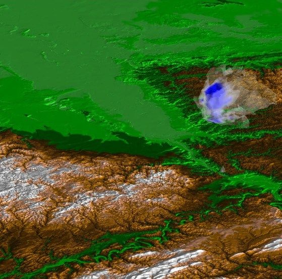
2                                            Gerstner et. al. / Visualization of Local Rainfall

                                                                         Figure 2: A schematic view of the weather radar scan grid.

Figure 1: A scenic view of the weather radar antenna on top
                                                                        the radar is not idle but scans only the smallest elevation
of a high building in Bonn, Germany.
                                                                        angle in a higher time resolution). The scanned volume is
                                                                        roughly 55,000 km3 covering about 7,900 km2 .
                                                                           The raw data sets have been obtained for a 1 degree reso-
tion models are built independently, they are constructed in            lution of the azimuth angle, for elevation angles of 1.5, 2.5,
a matching way. In our case, the 3D model is based on re-               3.5, 4.5, 6.0, 8.0, 10.0, and 12.0 degrees, and for 200 equidis-
cursive tetrahedral bisection and the 2D model is based on              tant points along each ray. In summary, each time–slice of
recursive triangle bisection. This way, in principle, visibil-          raw data consists of 360 × 200 × 9 floating point values.
ity problems which result from the merging of the data sets
might be solved as well. In our experience so far mutual vis-
ibility did not pose a real problem, though.                            3. Preprocessing of the Raw Data
   The employed volume visualization algorithm is based                 The raw radar data is prone to various sources of error and
on the simultaneous extraction of several transparent isosur-           thus has to be filtered before further processing. In this sec-
faces. This choice is motivated by the experience that the              tion we will shortly illustrate the various necessary steps.
display of isosurfaces appears to be more meaningful to peo-
ple from the atmospheric sciences than direct volume render-
                                                                        3.1. Clutter Filtering
ing. As an added benefit, no special–purpose hardware (apart
from a standard graphics card) has to be used.                          Clutter are unwanted signals, e.g. resulting from reflections
                                                                        at non–meteorological obstacles such as mountains, build-
   The outline of this paper is as follows. In Section 2 we will
                                                                        ings, and industrial plants (ground clutter), or at birds and
give some technical details on the weather radar device and
                                                                        airplanes (moving clutter). Such obstacles alter the signal not
the derived data. Section 3 covers the preprocessing of the
                                                                        only at their location, but also behind them with respect to
data. The multiresolution algorithm is explained in Section
                                                                        the position of the antenna.
4. In Section 5 we will illustrate the performance of the sys-
tem with some examples. We conclude with a few remarks                     The basic way to filter the ground clutter is to record the
on further extensions in Section 6.                                     measured signals on a dry day in a so called cluttermap. The
                                                                        cluttermap will be subtracted from the operationally mea-
                                                                        sured signals. Thereby, each measured reflectivity value is
2. About the Weather Radar
                                                                        compared to its pendant of the cluttermap. Values with pre-
The radar antenna† is mounted on top of a 7–storey resi-                cipitation are reduced if they are supposed to be contami-
dential building in Bonn (geographical position 70◦ 040 E,              nated by clutter. Afterwards, a weak low pass filter is applied
50◦ 430 N) in a height of 98.5 meters over sea level. It is             to the image to eliminate residual clutter signals due to ap-
operated in a continuous mode (save maintenance). The an-               parent displacement of ground echoes caused by variations
tenna is able to rotate 360 degrees around its vertical axis            of the refractive index within the atmosphere13 . An exam-
(azimuth angle) and tilt up to 90 degrees with respect to the           ple for the behaviour of the clutter filtering algorithm for a
horizontal plane (elevation angle). For each combination of             single scan of the second lowest elevation angle is shown in
azimuth and elevation angle reflectivities along the shot ray           Figure 3.
are obtained. The measurement radius is 50 km.
  A circular scan for each elevation angle forms an – albeit            3.2. Attenuation Correction
very flat – cone (see Figure 2). One complete 3D scan takes
                                                                        When hydrometeors reflect the energy of the pulse sent by
5 minutes and is repeated every 30 minutes (in the meantime
                                                                        the antenna, they also weaken the incoming pulse for the fol-
                                                                        lowing volumes. This is not considered in the radar equation
† type Selenia METEOR–200                                               but can be corrected successively for each measured ray6 .

                                                                          submitted to Joint EUROGRAPHICS - IEEE TCVG Symposium on Visualization (2002)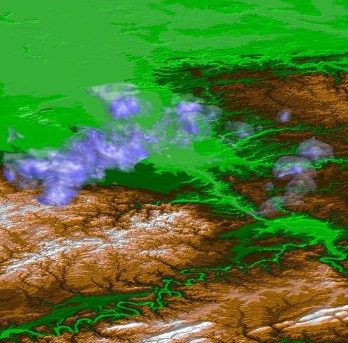
Gerstner et. al. / Visualization of Local Rainfall                                         3

                                                                                   Figure 4: The recursive bisection hierarchy in 2D and in
                                                                                   3D. The upper row shows the respective refinement rules,
Figure 3: 2D plots of the rainfall data for the second low-                        the lower row the initial grids and the first refinement step.
est elevation angle: original measurements and after clutter
filtering.

                                                                                   4. Multiresolution Visualization
                                                                                   The here used multiresolution visualization algorithms
But, because attenuation affects the signal just in case of very
                                                                                   (both in 2D and 3D) have been presented in previous
strong precipitation and this kind of correction is very sensi-
                                                                                   publications3, 4 . At this point, we will just repeat the main
tive to measurements errors, it is employed in special cases
                                                                                   steps in order to illustrate the special adaptions required for
only (as in the example of Section 5.1).
                                                                                   the application under consideration.

3.3. Z–R Relationship                                                              4.1. Multiresolution Hierarchy
The receiver of the radar system measures the power of the                         Let us consider a hierarchy of triangular, respectively tetra-
reflected pulse. To relieve the measurements from their de-                        hedral grids generated by recursive bisection. To this end, the
pendency on range and the properties of the radar system, the                      midpoint of a predetermined edge is chosen as a refinement
data is usually converted into the so called radar reflectivity                    vertex and the triangle, respectively tetrahedron, is split in
(factor) Z. The link between Z and the rain rate R is called Z–                    two by connecting the refinement vertex with its opposing
R relationship and depends on the unknown drop size distri-                        vertices. Starting with initial meshes consisting of two trian-
bution within the illuminated volume. Using approximations                         gles, respectively six tetrahedra, and recursively splitting all
for the drop size distribution and the fall velocity formulas                      triangles or tetrahedra, nested hierarchical meshes are con-
of the form Z = aRb can be derived. We have used a = 300                           structed (Figure 4).
and b = 1.5 for our examples10 .
                                                                                      An adaptive mesh can be extracted from such a hierar-
                                                                                   chy by selection and computation of a suited error indicator.
3.4. Interpolation                                                                 Then, all triangles, respectively tetrahedra, whose associated
                                                                                   error indicator is below a user–prescribed error threshold are
As illustrated in Section 2, the raw data is given in a conical                    visited. If this error indicator is saturated then the result-
coordinate system. Although the data could be visualized in                        ing adaptive meshes cannot contain so–called hanging nodes
this coordinate system, this is impractical for two reasons.                       which would lead to holes during the visualization4, 17 .
First, it would be hard to match the three–dimensional mesh
with the two–dimensional terrain grid. This would be nec-
essary for the solution of mutual visibility problems of the                       4.2. Terrain Visualization
rainfall and terrain data. Second, the conical mesh is circu-
                                                                                   For a two–dimensional scalar field, such as terrain, it is suf-
lar along the azimuth angle and thus not homeomorphic to a
                                                                                   ficient to draw and shade the triangles on the finest local
cubical mesh. This would require a special treatment of the
                                                                                   resolution. An often applied extension is view–dependent
circularity which is difficult.
                                                                                   refinement12 which is usually used for low flyovers. Here,
   In order to avoid these problems, we interpolated the data                      the error threshold is not uniformly distributed but increases
set onto a cubical grid with 400 × 400 × 66 grid points us-                        with the distance to the viewer. For this application, view–
ing trilinear interpolation. In comparison to the conical grid,                    dependent refinement was not necessary since, due to the
the resolution of the cubical grid is about a factor of two                        nature of the data, a top or bird’s view is mostly used (com-
higher in lateral direction and a factor of seven higher in ele-                   pare Figure 6). For visualization purposes the triangles are
vation direction in order to minimize the interpolation error.                     color shaded according to elevation value using a simple ge-
Though the interpolated data set is about 16 times larger than                     ographical colormap ranging from green (low elevation) to
the raw data, it is much easier to handle.                                         white (high elevation).

submitted to Joint EUROGRAPHICS - IEEE TCVG Symposium on Visualization (2002)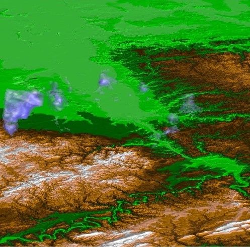
4 Gerstner et. al. / Visualization of Local Rainfall
4.3. Rainfield Visualization
Three–dimensional scalar fields require special volume vi-
sualization techniques such as volume rendering (e.g. us-
ing tetrahedral splats15 ) or isosurface extraction (e.g. using
marching tetrahedra14 ). Isosurfaces can be efficiently ex-
tracted hierarchically if additionally bounds for the mini-
mum and maximum data value inside each tetrahedron are Figure 5: The mutual occlusion problem: part of the rain-
available. The extraction algorithm then traverses the hierar- field is located in between two mountains. Rendering the
chical mesh searching only through those regions where the opaque terrain first and then the transparent rainfield does
isosurface is actually located (see Figure 7) and extracts the not lead to correct results. In principle, an interleaved
local isosurface using a simple lookup–table on the finest lo- traversal of the terrain and rainfield meshes is required.
cal resolution17 . Multiple transparent isosurfaces can be ren-
dered using alpha blending if the tetrahedra and isosurface
components are sorted in visibility order3 . However, the coupling of the two error thresholds has to
In our examples, we visualize the rainfall by 20 trans- be addressed. Although the two thresholds could be cho-
parent isosurfaces with low opacity and color ranging from sen independently, the user should not have to adjust both
white (low rainfall) to blue (high rainfall). The isovalues are of then. We solved the problem here by providing the user
equidistant and the maximum isovalue is determined by the with a global error ruler and a second ruler which controls
maximum rainfall in the data set (single event), respectively the relation between the the two errors. This way, the user
the maximum rainfall during the time interval (time series). will adjust the accurracy of the terrain in comparison to the
The isosurface triangles are Gouraud shaded based on the rainfield once, and use a global error ruler to control fidelity.
gradients of the 3D data set. Latter threshold could be determined automatically based on
the performance, but we did not feel it necessary here.
4.4. Integration
5. Examples
In this application, the user focus is clearly on the rainfield.
The terrain is mainly displayed for orientation and spatial We will now illustrate the performance and results of the
analysis. Nevertheless, the terrain has to cover a far greater visualization tool with some examples. The first example
area than the extent of the radar on the ground in order to shows a single rainfall event while the second example cov-
be able to also provide realistic side views of the rainfield. ers a time series. In all examples the rainfall data is displayed
In our experience, the terrain should extend at least twice on top of a 50 m digital elevation model‡ of roughly three
the rainfield size in all directions. This way, however, the times the extent of the measurement area. The height of the
two meshes cannot be constructed in a matching way in the terrain data as well as the rainfield data is exaggerated by a
sense that the z–projection of the 3D mesh will fall exactly factor of 5 in the images. Of course, the height exaggeration
onto the 2D mesh. can be controlled by the user but this value proved to be the
most useful.
In principle, intervisibility between the two data sets is a
problem due to the transparency of the isosurfaces which re-
quires alpha blending. For example, if part of the rainfield 5.1. Single Event
is located in between two mountains, then the more distant We will start with a highly localized and heavy rainfall event
mounain has to be drawn first, then the rainfield, and the which occurred during May 3rd, 2001. This event is impor-
closer mountain last (see Figure 5). This case can occur since tant since it caused severe damage in the region. The spatial
the viewing direction does not have to be identical to the di- extent of the event on the ground is roughly 100 km2 .
rection of the radar ray. However, it did not pose a real prob-
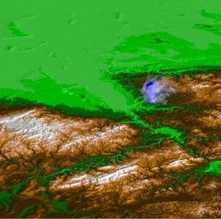
lem here since, due to the nature of the radar, the measured Figure 6 (a) depicts the location of the measurement area
rainfield is usually located high above the ground (compare of the radar in northwestern Germany. In Figure 6 (b) this
Figure 6d). The problem per se is interesting though and area (circular with 100 km diameter) as viewed from di-
would require an interleaved traversal of the two multireso- rectly above is shown. In the center is the city of Bonn,
lution hierarchies which is not a trivial problem and subject the river Rhine runs from southeast (Koblenz) to northwest
to current research. (Cologne). Note that this top view is already more illus-
trative to the meteorologist than single horizontal slices (as
Due to these two problems we treat the rainfield and the Figure 3). The 3D structure of the rainfall is really revealed
terrain meshes independently from each other as two sep- through interactive rotation and movement through the data
arate multiresolution hierarchies. In order to achieve suffi-
ciently correct results the terrain is rendered first and the
rainfield field second. ‡ courtesy of SFB350, University of Bonn
submitted to Joint EUROGRAPHICS - IEEE TCVG Symposium on Visualization (2002)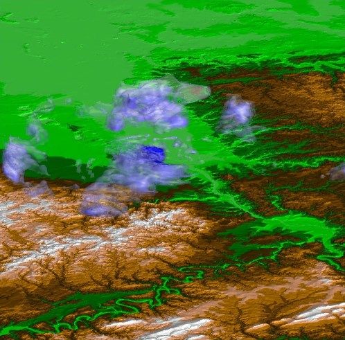
Gerstner et. al. / Visualization of Local Rainfall 5
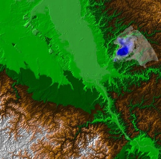
set. As an example, Figure 6 (c) shows a 70 degree angle Here multiresolution algorithms were necessary in order to
view of the area. A closeup of the rainfall event as seen from be able to handle the large amounts of data in an interactive
a flat 87 degree angle facing northwest is shown in Figure 6 visualization environment.
(d). Here, the typical formation of rain tubes can be seen. On
We are currently working on further improvements of the
the upper border aliasing artefacts which result from the em-
visualization system such as the inclusion of symbols and
ployed interpolation algorithm (see Section 3.4) are visible.
rainfall animation. Certainly a great improvement would be
In Figure 7 we show the multiresolution performance of a multiresolution hierarchy on the native (conical) coordi-
the visualization system. Here we show the corresponding nate system of the radar measurements, because this way
triangular and tetrahedral grids next to the terrain and rain- interpolation errors and aliasing artefacts can be avoided.
field. From left to right the global error threshold (see Sec- This, however, will require special visualization algorithms
tion 4.4) was decreased by a factor of ten resulting in an for cyclic meshes, and visibility problems will be still harder
increase of the number of triangles also by a factor of ten to solve. Also, 3D data compression schemes which allow
(in this example, the number of isosurface and terrain tri- the visualization based on compressed rainfall data will be
angles were roughly the same). As can be seen, the isosur- an interesting research direction.
face extraction algorithm refines only in the vicinity of the
isosurface. The terrain is also much coarser in smooth, less Acknowledgement
mountainous areas such as in the upper part of the images
which substantially increases the overall performance. For The authors would like to thank SFB 350 ”Interaction be-
the coarser images in addition the number of displayed iso- tween and modeling of continental geosystems” of the Ger-
surfaces were reduced to 5, respectively 10. This number man research foundation (DFG) for previous financial sup-
was also coupled to the global error threshold. port.
The whole system is interactive for large error thresholds
(as in Figure 7 left and middle) while higher resolution im- References
ages (such as Figure 7 right) require a few seconds rendering 1. P. Chen. Climate and Weather Simulations and Data Vi-
time on an Intel Pentium III with a standard nVidia graphics sualization using a Supercomputer, Workstations, and
card running Linux. For the rightmost image several million Microcomputers. In Visual Data Exploration and Anal-
triangles were rendered. ysis III (Proc. SPIE ’95), volume 2656, pages 254–264.
SPIE, 1996.
5.2. Time Series 2. J. Doick and A. Holt. The Full Volume Simultane-
As a second example will serve a heavy convective rainfall ous Visualization of Weather Radar Echoes with Dig-
event which has occurred on July 20th, 2001. In Figure 8 we ital Terrain Map Data. In R. Earnshaw, J. Vince, and
show three images at 11:52, 12:22, and 12:52. The wind di- H. Jones, editors, Visualization and Modeling, pages
rection is from the southwest and thus the rain front moves 73–86. Academic Press, 1997.
roughly from left to right in the images. Well visible here is 3. T. Gerstner. Fast Multiresolution Extraction of Multi-
the deficiency that the radar does not cover the area directly ple Transparent Isosurfaces. In D. Ebert, J. Favre, and
above the antenna (which is located in the middle of the im- R. Peikert, editors, Data Visualization ’01, pages 35–
ages). This problem could be solved by increasing the max- 44. Springer, 2001.
imum elevation angle, or using several radar devices with
overlapping measurement areas. 4. T. Gerstner, M. Rumpf, and U. Weikard. Error Indi-
cators for Multilevel Visualization and Computing on
For larger time series the rainfall data should be stored
Nested Grids. Computers & Graphics, 24(3):363–373,
in compressed form (not only on disk but also in memory).
2000.
Since large parts of the rainfield are typically empty (zero
rainfall) this can be achieved by the construction of adap- 5. H. Haase, M. Bock, E. Hergenröther, C. Knöpfle, H.-
tive tetrahedral meshes which capture the rain data (such as J. Koppert, F. Schröder, A. Trembilski, and J. Wei-
in Figure 7 lower right). Then, only the data values in the denhausen. Meteorology Meets Computer Graphics
adaptive mesh together with the corresponding tree structure – A Look at a Wide Range of Weather Visualiza-
(which requires only a few bits per vertex) have to be stored. tions for Diverse Audiences. Computers & Graphics,
However, this was not necessary for the small time series in 24(3):391–397, 2000.
the example. 6. S. Hacker. Probleme mit der Dämpfungskorrektur von
Radardaten. Master’s thesis, Meteorological Institute,
6. Concluding Remarks University of Bonn, 1996.
We have illustrated a meteorological application of volume 7. W. Hibbard, J. Anderson, I. Foster, B. Paul, R. Ja-
visualization for rainfall measurements from weather radar. cob, C. Schafer, and M. Tyree. Exploring coupled
submitted to Joint EUROGRAPHICS - IEEE TCVG Symposium on Visualization (2002)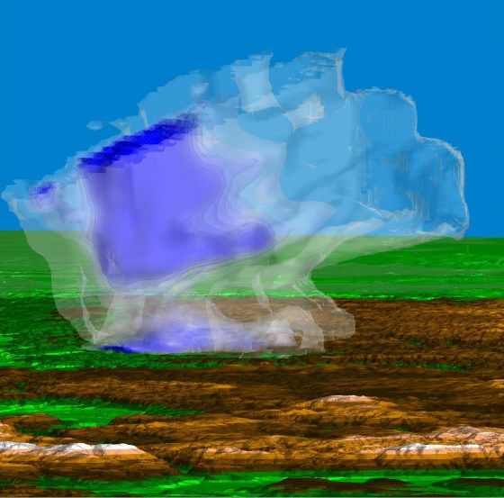
6                                            Gerstner et. al. / Visualization of Local Rainfall

     Atmosphere–Ocean Models using Vis5D. Interna-
     tional Journal of Supercomputing Applications and
     High Performance Computing, 10(2):211–222, 1996.
8.   C. James, S. Brodzik, H. Edmon, R. Houze Jr, and
     S. Yuter. Radar Data Processing and Visualization over
     Complex Terrain. Weather and Forecasting, 15:327–
     338, 2000.
9.   T. Jiang, W. Ribarsky, T. Wasilewski, N. Faust, B. Han-
     nigan, and M. Parry. Acquisition and Display of Real–
     Time Atmospheric Data on Terrain. In D. Ebert,
     J. Favre, and R. Peikert, editors, Data Visualization ’01,
     pages 15–24. Springer, 2001.
10. J. Joss and A. Waldvogel. A Method to Improve the Ac-
    curacy of Radar-Measured Amounts of Precipitation.
    In Proc. 14th International Conference on Radar Mete-
    orology, pages 237–238. American Meteorological So-
    ciety, 1970.
11. D. Koller, P. Lindstrom, W. Ribarsky, L. Hodges,
    N. Faust, and G. Turner. Virtual GIS: A Real–Time
    3D Geographic Information System. In Proceedings
    IEEE Visualization ’95, pages 94–100. IEEE Computer
    Society Press, 1995.
12. P. Lindstrom, D. Koller, W. Ribarsky, L. Hodges,
    N. Faust, and G. Turner. Real–Time, Continuous
    Level of Detail Rendering of Height Fields. Computer
    Graphics (SIGGRAPH ’96 Proceedings), pages 109–
    118, 1996.
13. D. Meetschen. Erkennung, Nutzung und Entfernung
    von Clutter zur Verbesserung der Niederschlagsmes-
    sung mit dem Bonner Radar. Master’s thesis, Meteo-
    rological Institute, University of Bonn, 1999.
14. B. Payne and A. Toga. Surface Mapping Brain Function
    on 3D Models. IEEE Computer Graphics and Applica-
    tions, 10(5):33–41, 1990.
15. P. Shirley and A. Tuchman. A Polygonal Approxima-
    tion to Direct Scalar Volume Rendering. ACM Com-
    puter Graphics (Proc. of Volume Visualization ’90),
    24(5):63–70, 1990.
16. M. Toussaint, M. Malkomes, M. Hagen, H. Höller, and
    P. Meischner. A Real–Time Visualization, Analysis
    and Management Toolkit for Multi–Parameter, Multi–
    Static Weather Radar Data. In Proc. 30th Interna-
    tional Conference on Radar Meteorology, pages 56–57.
    American Meteorological Society, 2001.
17. Y. Zhou, B. Chen, and A. Kaufman. Multiresolution
    Tetrahedral Framework for Visualizing Volume Data.
    In Proc. IEEE Visualization ’97, pages 135–142. IEEE
    Computer Society Press, 1997.

                                                                          submitted to Joint EUROGRAPHICS - IEEE TCVG Symposium on Visualization (2002)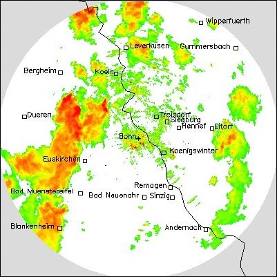
Gerstner et. al. / Visualization of Local Rainfall                   7

                                  (a) Location                                                             (b) Top view

                                  (c) Bird’s view                                                          (d) Closeup
Figure 6: Four images visualizing a heavy local rainfall event during May 3rd, 2001 in northwestern Germany. Displayed is
the terrain and 20 transparent isosurfaces with low opacity and color ranging from white to blue. All heights are exaggerated
by a factor of 5.

submitted to Joint EUROGRAPHICS - IEEE TCVG Symposium on Visualization (2002)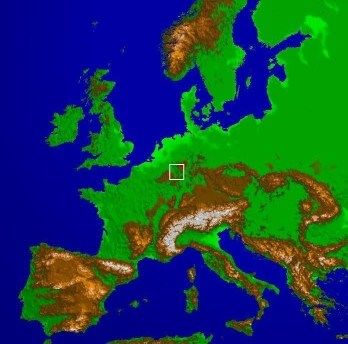
8                                          Gerstner et. al. / Visualization of Local Rainfall

Figure 7: The multiresolution approach for the terrain as well as for the isosurfaces allows scalable performance for the
interaction with the data. The images show terrain and isosurface renderings as well as the corresponding 2D and 3D grids for
varying error thresholds. The number of triangles and tetrahedra increase by a factor of 10 in between the images.

Figure 8: Three snapshots of a heavy convective rainfall event on July 20th, 2001 (moving from left to right). The time between
the images is 30 minutes. Note that directly above the radar antenna (in the middle of the images) no rainfall information is
available.

                                                                        submitted to Joint EUROGRAPHICS - IEEE TCVG Symposium on Visualization (2002)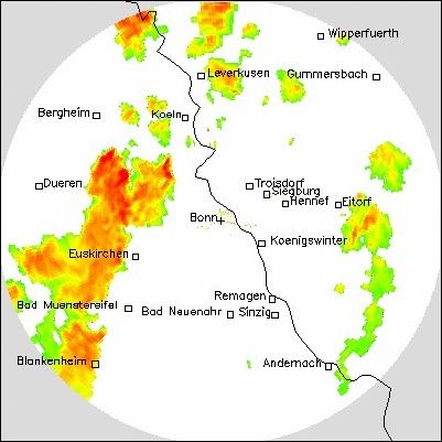
You can also read